Atazanavir + Ritonavir (Molto 2016)
Source:vignettes/articles/Molto_2016_atazanavir_ritonavir.Rmd
Molto_2016_atazanavir_ritonavir.RmdModel and source
- Citation: Molto J, Estevez JA, Miranda C, Cedeno S, Clotet B, Valle M. Population pharmacokinetic modelling of the changes in atazanavir plasma clearance caused by ritonavir plasma concentrations in HIV-1 infected patients. Br J Clin Pharmacol. doi:10.1111/bcp.13072.
- Description: Simultaneous one-compartment popPK model for oral atazanavir (ATV, parent / substrate) and ritonavir (RTV, sibling-drug suffix _rtv) in 83 HIV-1-infected Caucasian adults receiving either ATV 400 mg or ATV 300 mg + RTV 100 mg once daily. Both drugs use a Savic transit- compartment absorption chain (ATV: N = 7, MTT = 0.80 h, ka = 2.05 1/h; RTV: N = 11, MTT = 0.522 h, ka = 1.21 1/h) feeding a depot, followed by first-order elimination from a one-compartment central. ATV apparent clearance is exponentially inhibited by RTV plasma concentration: CL/F_ATV(t) = exp(lcl) * exp(-e_crtv_cl * C_RTV(t)) with the unboosted CL/F_ATV = 11.7 L/h and inhibition coefficient 0.296 L/mg. This functional form reproduces the paper’s reported ~18% reduction in ATV CL at the cohort-mean RTV concentration of 0.63 mg/L and explains 17.5% of inter-individual variability in ATV CL. Demographic covariates (weight allometric, gender, age, TDF, HCV, dose-timing, AAG, albumin) were screened by GAM and tested in NONMEM but not retained; an Emax-form and a linear-form inhibition were also tested and rejected (Emax: unrealistic estimates; linear: biased fit). IIV on ka / CL/F / V/F is reported for both drugs with unusually large IIV on absorption (~200% CV) confirmed in the paper Results. ATV residual error is combined (27.0% proportional + 0.07 mg/L additive); RTV residual error is proportional only (28.0%; the additive component of the initial combined error was deleted as negligible) (Molto 2016).
- Article: https://doi.org/10.1111/bcp.13072
Population
Molto 2016 enrolled 83 HIV-1-infected Caucasian adults at a single Spanish centre (Hospital Universitari Germans Trias i Pujol, Badalona, Catalonia) between May 2004 and May 2009. Patients were on stable antiretroviral therapy for at least four weeks at sampling so the model is fitted under steady-state conditions. 53/83 patients received boosted ATV (300 mg + RTV 100 mg once daily); the remaining 30 received unboosted ATV (400 mg once daily). Median age 42 years (range 26-75); median body weight 70 kg (range 40-91); 68.67% male (31.33% female). 38/83 patients (45.78%) were also receiving tenofovir 300 mg once daily. 30/83 (36.14%) had HCV coinfection but only 5/83 (6.02%) had advanced liver fibrosis (Molto 2016 Table 1).
Several demographic and clinical covariates (weight via allometric scaling, gender, age, HCV coinfection, tenofovir co-administration, dose timing morning-vs-night, and the laboratory parameters AST, ALT, AAG, albumin) were tested in NONMEM after preselection by GAM. None was retained in the final model; the only structural perturbation that survived was the exponential inhibition of ATV CL by ritonavir plasma concentration. The packaged model therefore exposes no covariate columns.
The same information is available programmatically via
readModelDb("Molto_2016_atazanavir_ritonavir")()$meta$population.
Source trace
Per-parameter origin is recorded as an in-file comment next to each
ini() entry in
inst/modeldb/specificDrugs/Molto_2016_atazanavir_ritonavir.R.
The table below collects them for review.
| Equation / parameter | Value | Source location |
|---|---|---|
| Atazanavir ka | 2.05 1/h (RSE 19.5%) | Table 2, “Final model” |
| Atazanavir MTT | 0.80 h (RSE 6.2%) | Table 2, “Final model” |
| Atazanavir N transit (FIXED) | 7 | Table 2, “Final model” (integer; no RSE) |
| Atazanavir CL/F (unboosted) | 11.7 L/h (RSE 6.8%) | Table 2, “Final model” |
| Atazanavir V/F | 95.7 L (RSE 6.5%) | Table 2, “Final model” |
| Ritonavir ka | 1.21 1/h (RSE 24.7%) | Table 2, “Final model” |
| Ritonavir MTT | 0.522 h (RSE 3.8%) | Table 2, “Final model” |
| Ritonavir N transit (FIXED) | 11 | Table 2, “Final model” (integer; no RSE) |
| Ritonavir CL/F | 9.68 L/h (RSE 3.0%) | Table 2, “Final model” |
| Ritonavir V/F | 70.5 L (RSE 8.8%) | Table 2, “Final model” |
| theta_C(RTV),CL/F (exponential inhibition coefficient) | 0.296 L/mg (RSE 3.5%) | Table 2, “Final model” |
| IIV ka_ATV | 200.2% CV (RSE 22.4%) | Table 2, “Final model” |
| IIV CL/F_ATV | 57.4% CV (RSE 18.1%) | Table 2, “Final model” |
| IIV V/F_ATV | 37.4% CV (RSE 21.4%) | Table 2, “Final model” |
| IIV ka_RTV | 207.8% CV (RSE 26.1%) | Table 2, “Final model” |
| IIV CL/F_RTV | 60.0% CV (RSE 27.7%) | Table 2, “Final model” |
| IIV V/F_RTV | 49.0% CV (RSE 29.1%) | Table 2, “Final model” |
| Atazanavir proportional residual | 27.0% (RSE 7.4%) | Table 2, “Final model” |
| Atazanavir additive residual | 0.07 mg/L (RSE 14.2%) | Table 2, “Final model” |
| Ritonavir proportional residual | 28.0% (RSE 3.5%) | Table 2, “Final model” |
| Exponential inhibition equation | CL_ATV(t) = exp(lcl) * exp(-e_crtv_cl * C_RTV(t)) |
Methods, “Final model” paragraph |
| Savic transit absorption form | transit(n, MTT, F=1) -> depot -> ka * depot -> central |
Methods, “Basic models for ATV and RTV” |
Virtual cohort
Original observed data are not publicly available. The simulations below build virtual cohorts of 200 subjects per dosing regimen covering the two real-world arms of the study (ATV 400 mg unboosted; ATV 300 mg + RTV 100 mg boosted) plus the two unlicensed once-daily reduction regimens that the paper highlights as worthy of further clinical evaluation (ATV 300 mg + RTV 50 mg; ATV 200 mg + RTV 100 mg). All four regimens are dosed for 10 consecutive days so steady state is achieved at the day-10 dosing interval (atazanavir terminal half-life of ~6 h with no accumulation). Subjects have no covariates beyond ID because the final model retains no covariate effects.
set.seed(20260620)

n_per_arm <- 200L
tau       <- 24                      # dosing interval (h)
n_doses   <- 10L                     # 10 daily doses -> steady state
dose_times <- seq(0, by = tau, length.out = n_doses)
day10_start <- (n_doses - 1) * tau

obs_times <- sort(unique(c(
  seq(0,                   tau,                length.out = 25),  # dense day-1 interval
  seq(tau,                 day10_start,        by         = tau), # daily troughs
  day10_start + seq(0, tau, length.out = 49)                       # dense day-10 interval
)))

regimens <- tibble::tribble(
  ~regimen,                 ~atv_mg, ~rtv_mg,
  "ATV 400 mg QD",              400,       0,
  "ATV 300/RTV 100 mg QD",      300,     100,
  "ATV 300/RTV 50 mg QD",       300,      50,
  "ATV 200/RTV 100 mg QD",      200,     100
)

make_cohort <- function(n, atv_mg, rtv_mg, regimen, id_offset) {
  ids <- id_offset + seq_len(n)

  dose_atv <- tidyr::expand_grid(id = ids, time = dose_times) |>
    dplyr::mutate(amt = atv_mg, cmt = "depot", evid = 1L)

  rows <- dose_atv

  # Only add ritonavir dose rows when RTV is part of the regimen.
  if (rtv_mg > 0) {
    dose_rtv <- tidyr::expand_grid(id = ids, time = dose_times) |>
      dplyr::mutate(amt = rtv_mg, cmt = "depot_rtv", evid = 1L)
    rows <- dplyr::bind_rows(rows, dose_rtv)
  }

  # Observations on the algebraic observables Cc (ATV) and Cc_rtv (RTV) so
  # the rxode2 dvid mapping resolves cleanly in the multi-output model.
  obs <- tidyr::expand_grid(id = ids, time = obs_times,
                            cmt = c("Cc", "Cc_rtv")) |>
    dplyr::mutate(amt = 0, evid = 0L)

  dplyr::bind_rows(rows, obs) |>
    dplyr::mutate(regimen = regimen) |>
    dplyr::arrange(id, time, dplyr::desc(evid))
}

id_seed <- 0L
events_list <- vector("list", nrow(regimens))
for (i in seq_len(nrow(regimens))) {
  r <- regimens[i, ]
  events_list[[i]] <- make_cohort(n_per_arm, r$atv_mg, r$rtv_mg, r$regimen,
                                  id_offset = id_seed)
  id_seed <- id_seed + n_per_arm
}
events <- dplyr::bind_rows(events_list)
stopifnot(!anyDuplicated(unique(events[, c("id", "time", "evid", "cmt")])))
Simulation
mod <- readModelDb("Molto_2016_atazanavir_ritonavir")

# Stochastic VPC with the published IIV.
sim <- rxode2::rxSolve(mod, events = events, keep = c("regimen")) |>
  as.data.frame()
#> ℹ parameter labels from comments will be replaced by 'label()'

# Deterministic (typical-value) profiles for figure replication.
mod_typical <- rxode2::zeroRe(mod)
#> ℹ parameter labels from comments will be replaced by 'label()'
sim_typical <- rxode2::rxSolve(mod_typical, events = events,
                               keep = c("regimen")) |>
  as.data.frame()
#> ℹ omega/sigma items treated as zero: 'etalka', 'etalcl', 'etalvc', 'etalka_rtv', 'etalcl_rtv', 'etalvc_rtv'
#> Warning: multi-subject simulation without without 'omega'
Replicate published figures
Figure 1 (boosted vs unboosted ATV) – steady-state profile
Molto 2016 Figure 1 plots observed ATV plasma concentrations across the 24-h dosing interval at steady state for ATV 400 mg QD (unboosted) and ATV 300 mg + RTV 100 mg QD (boosted). The packaged model is exercised on a typical-value (no-IIV) curve overlaid on a stochastic envelope so the reduced ATV CL from RTV co-administration shows clearly as a higher boosted-arm trough at the same nominal dose level.
day10 <- sim |>
  dplyr::filter(time >= day10_start) |>
  dplyr::mutate(t_h = time - day10_start)
day10_typ <- sim_typical |>
  dplyr::filter(time >= day10_start) |>
  dplyr::mutate(t_h = time - day10_start)

vpc_atv <- day10 |>
  dplyr::group_by(regimen, t_h) |>
  dplyr::summarise(
    Q05 = quantile(Cc, 0.05, na.rm = TRUE),
    Q50 = quantile(Cc, 0.50, na.rm = TRUE),
    Q95 = quantile(Cc, 0.95, na.rm = TRUE),
    .groups = "drop"
  )
typ_atv <- day10_typ |>
  dplyr::distinct(regimen, t_h, Cc)

ggplot() +
  geom_ribbon(data = vpc_atv,
              aes(t_h, ymin = Q05, ymax = Q95, fill = regimen),
              alpha = 0.20) +
  geom_line(data = vpc_atv, aes(t_h, Q50, colour = regimen), linewidth = 0.6) +
  geom_line(data = typ_atv, aes(t_h, Cc, colour = regimen),
            linewidth = 1.0, linetype = "dashed") +
  scale_y_log10() +
  labs(x = "Time after dose (h)",
       y = "Atazanavir plasma concentration (mg/L)",
       title = "Figure 1 -- ATV steady-state profile by regimen",
       caption = paste0("Replicates Figure 1 of Molto 2016. Solid line: ",
                        "stochastic median (n = ", n_per_arm,
                        " per regimen). Dashed line: typical-value profile. ",
                        "Ribbon: 5th-95th percentile."))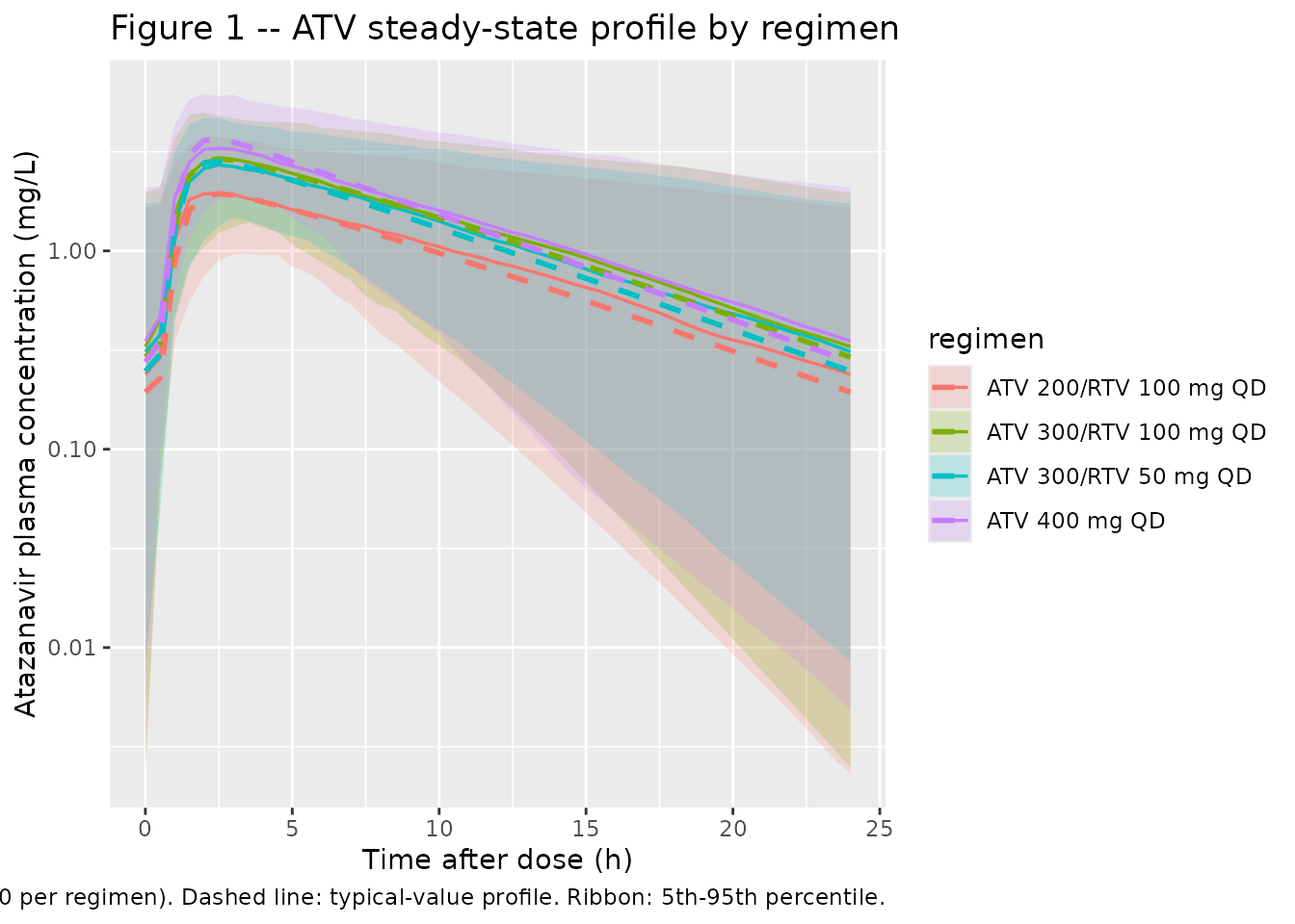
Figure 2 – ritonavir steady-state profile
Molto 2016 Figure 2 plots observed RTV plasma concentrations across the 24-h dosing interval at steady state. The packaged model reproduces a typical-value and stochastic envelope for the boosted ATV 300/RTV 100 mg regimen.
day10_rtv <- day10 |> dplyr::filter(regimen != "ATV 400 mg QD")
day10_rtv_typ <- day10_typ |> dplyr::filter(regimen != "ATV 400 mg QD")

vpc_rtv <- day10_rtv |>
  dplyr::group_by(regimen, t_h) |>
  dplyr::summarise(
    Q05 = quantile(Cc_rtv, 0.05, na.rm = TRUE),
    Q50 = quantile(Cc_rtv, 0.50, na.rm = TRUE),
    Q95 = quantile(Cc_rtv, 0.95, na.rm = TRUE),
    .groups = "drop"
  )
typ_rtv <- day10_rtv_typ |>
  dplyr::distinct(regimen, t_h, Cc_rtv)

ggplot() +
  geom_ribbon(data = vpc_rtv,
              aes(t_h, ymin = Q05, ymax = Q95, fill = regimen),
              alpha = 0.20) +
  geom_line(data = vpc_rtv, aes(t_h, Q50, colour = regimen), linewidth = 0.6) +
  geom_line(data = typ_rtv, aes(t_h, Cc_rtv, colour = regimen),
            linewidth = 1.0, linetype = "dashed") +
  scale_y_log10() +
  labs(x = "Time after dose (h)",
       y = "Ritonavir plasma concentration (mg/L)",
       title = "Figure 2 -- RTV steady-state profile by regimen",
       caption = paste0("Replicates Figure 2 of Molto 2016. Solid line: ",
                        "stochastic median. Dashed line: typical-value. ",
                        "Ribbon: 5th-95th percentile."))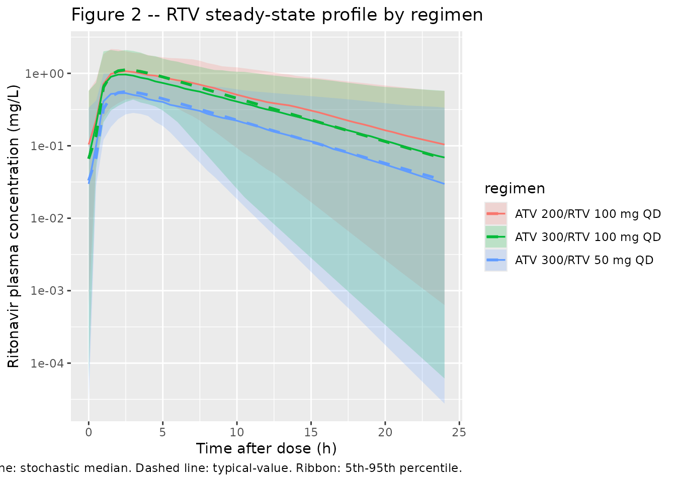
Inhibition curve
A short sanity check on the exponential inhibition factor: at the cohort- mean RTV plasma concentration of 0.63 mg/L the model predicts a 17.0% reduction in ATV CL/F. The paper Results paragraph rounds this to “an 18% decrease”, consistent within the rounding precision of the cited mean RTV concentration.
crtv_grid <- seq(0, 1.5, length.out = 200)
e_crtv_cl <- 0.296
inhib_df <- tibble::tibble(
  C_RTV   = crtv_grid,
  factor  = exp(-e_crtv_cl * crtv_grid),
  pct_red = 100 * (1 - factor)
)
mean_crtv <- 0.63
inhib_at_mean <- 100 * (1 - exp(-e_crtv_cl * mean_crtv))

ggplot(inhib_df, aes(C_RTV, pct_red)) +
  geom_line(linewidth = 0.8) +
  geom_vline(xintercept = mean_crtv, linetype = "dotted") +
  geom_hline(yintercept = inhib_at_mean, linetype = "dotted") +
  labs(x = "Ritonavir plasma concentration (mg/L)",
       y = "Predicted reduction in ATV CL/F (%)",
       title = "ATV CL/F reduction as a function of RTV plasma concentration",
       caption = paste0(
         "At the cohort-mean C_RTV = 0.63 mg/L, the model predicts ",
         sprintf("%.1f%%", inhib_at_mean),
         " reduction in ATV CL/F (paper rounds to 18%)."))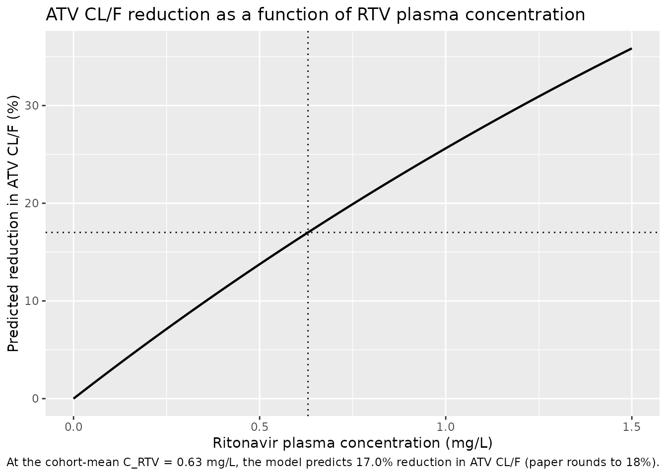
PKNCA validation
PKNCA computes steady-state Cmax, Cmin, Cav, and AUC0-tau over the
final (day-10) dosing interval for ATV and RTV stratified by
regimen. The PKNCA formula uses regimen + id
so per-regimen summaries can be compared against any per-arm values
reported in the paper.
nca_window_atv <- sim |>
  dplyr::filter(time >= day10_start, time <= day10_start + tau) |>
  dplyr::filter(!is.na(Cc)) |>
  dplyr::distinct(id, time, regimen, .keep_all = TRUE) |>
  dplyr::select(id, time, Cc, regimen)

dose_df_atv <- events |>
  dplyr::filter(evid == 1, cmt == "depot",
                time == max(time[evid == 1L & cmt == "depot"])) |>
  dplyr::distinct(id, time, amt, regimen)

conc_atv <- PKNCA::PKNCAconc(nca_window_atv,
                             Cc ~ time | regimen + id,
                             concu = "mg/L", timeu = "h")
dose_atv_obj <- PKNCA::PKNCAdose(dose_df_atv, amt ~ time | regimen + id,
                                 doseu = "mg")

intervals_ss <- data.frame(
  start   = day10_start,
  end     = day10_start + tau,
  cmax    = TRUE,
  cmin    = TRUE,
  tmax    = TRUE,
  auclast = TRUE,
  cav     = TRUE
)

nca_res_atv <- PKNCA::pk.nca(PKNCA::PKNCAdata(conc_atv, dose_atv_obj,
                                              intervals = intervals_ss))
nca_summary_atv <- as.data.frame(summary(nca_res_atv))
knitr::kable(nca_summary_atv,
caption = "Simulated steady-state NCA -- atazanavir, by regimen.")| Interval Start | Interval End | regimen | N | AUClast (h*mg/L) | Cmax (mg/L) | Cmin (mg/L) | Tmax (h) | Cav (mg/L) |
|---|---|---|---|---|---|---|---|---|
| 216 | 240 | ATV 200/RTV 100 mg QD | 200 | 21.9 [59.8] | 2.07 [38.6] | 0.143 [681] | 2.00 [1.50, 8.50] | 0.914 [59.8] |
| 216 | 240 | ATV 300/RTV 100 mg QD | 200 | 31.6 [59.0] | 2.97 [39.0] | 0.185 [2180] | 2.50 [1.50, 10.5] | 1.32 [59.0] |
| 216 | 240 | ATV 300/RTV 50 mg QD | 200 | 29.8 [55.1] | 2.80 [37.0] | 0.216 [428] | 2.50 [1.50, 9.00] | 1.24 [55.1] |
| 216 | 240 | ATV 400 mg QD | 200 | 35.6 [56.0] | 3.57 [35.4] | 0.206 [1420] | 2.50 [1.50, 8.50] | 1.48 [56.0] |
boosted_regimens <- setdiff(regimens$regimen, "ATV 400 mg QD")

nca_window_rtv <- sim |>
  dplyr::filter(regimen %in% boosted_regimens,
                time >= day10_start, time <= day10_start + tau) |>
  dplyr::filter(!is.na(Cc_rtv)) |>
  dplyr::distinct(id, time, regimen, .keep_all = TRUE) |>
  dplyr::select(id, time, Cc_rtv, regimen)

dose_df_rtv <- events |>
  dplyr::filter(evid == 1, cmt == "depot_rtv",
                regimen %in% boosted_regimens,
                time == max(time[evid == 1L & cmt == "depot_rtv"])) |>
  dplyr::distinct(id, time, amt, regimen)

conc_rtv <- PKNCA::PKNCAconc(nca_window_rtv,
                             Cc_rtv ~ time | regimen + id,
                             concu = "mg/L", timeu = "h")
dose_rtv_obj <- PKNCA::PKNCAdose(dose_df_rtv, amt ~ time | regimen + id,
                                 doseu = "mg")

nca_res_rtv <- PKNCA::pk.nca(PKNCA::PKNCAdata(conc_rtv, dose_rtv_obj,
                                              intervals = intervals_ss))
nca_summary_rtv <- as.data.frame(summary(nca_res_rtv))
knitr::kable(nca_summary_rtv,
caption = "Simulated steady-state NCA -- ritonavir, by regimen.")| Interval Start | Interval End | regimen | N | AUClast (h*mg/L) | Cmax (mg/L) | Cmin (mg/L) | Tmax (h) | Cav (mg/L) |
|---|---|---|---|---|---|---|---|---|
| 216 | 240 | ATV 200/RTV 100 mg QD | 200 | 11.2 [57.4] | 1.13 [45.2] | 0.0546 [1300] | 2.50 [1.00, 10.5] | 0.467 [57.4] |
| 216 | 240 | ATV 300/RTV 100 mg QD | 200 | 9.80 [62.9] | 1.04 [52.5] | 0.0319 [7150] | 2.50 [1.00, 9.50] | 0.408 [62.9] |
| 216 | 240 | ATV 300/RTV 50 mg QD | 200 | 5.22 [60.5] | 0.584 [42.0] | 0.0144 [8790] | 2.50 [1.00, 10.0] | 0.218 [60.5] |
Comparison against published Ctrough cutoff fractions
Molto 2016 Table 3 reports, for each regimen, the percentage of simulated patients whose ATV Ctrough fell below the 0.15 mg/L minimum-effective cutoff and above the 0.85 mg/L safety-relevant cutoff. The packaged model reproduces these fractions on 200 simulated subjects per regimen (vs. 1,000 in the original paper); minor noise in the lower-percentile estimates is expected at the smaller sample size.
troughs <- sim |>
  dplyr::filter(time == day10_start + tau) |>
  dplyr::group_by(regimen) |>
  dplyr::summarise(
    pct_below_0_15 = 100 * mean(Cc < 0.15, na.rm = TRUE),
    pct_above_0_85 = 100 * mean(Cc > 0.85, na.rm = TRUE),
    median_Cc      = median(Cc, na.rm = TRUE),
    .groups        = "drop"
  )

published <- tibble::tribble(
  ~regimen,                  ~published_below_0_15, ~published_above_0_85,
  "ATV 400 mg QD",                            25.7,                  27.4,
  "ATV 300/RTV 100 mg QD",                    24.5,                  26.2,
  "ATV 300/RTV 50 mg QD",                     26.7,                  22.6,
  "ATV 200/RTV 100 mg QD",                    30.3,                  16.6
)

comparison <- troughs |>
  dplyr::left_join(published, by = "regimen") |>
  dplyr::transmute(
    regimen,
    median_Cc_mgL          = round(median_Cc, 3),
    pct_below_0_15_sim     = round(pct_below_0_15, 1),
    pct_below_0_15_paper   = published_below_0_15,
    pct_above_0_85_sim     = round(pct_above_0_85, 1),
    pct_above_0_85_paper   = published_above_0_85
  )

knitr::kable(
  comparison,
  caption = paste0(
    "Simulated end-of-interval ATV concentration distribution vs Molto 2016 ",
    "Table 3. Cutoffs: 0.15 mg/L (minimum effective) and 0.85 mg/L (safety)."
  )
)| regimen | median_Cc_mgL | pct_below_0_15_sim | pct_below_0_15_paper | pct_above_0_85_sim | pct_above_0_85_paper |
|---|---|---|---|---|---|
| ATV 200/RTV 100 mg QD | 0.238 | 40.0 | 30.3 | 13.5 | 16.6 |
| ATV 300/RTV 100 mg QD | 0.329 | 33.5 | 24.5 | 24.0 | 26.2 |
| ATV 300/RTV 50 mg QD | 0.310 | 35.0 | 26.7 | 21.0 | 22.6 |
| ATV 400 mg QD | 0.351 | 30.5 | 25.7 | 26.0 | 27.4 |
Assumptions and deviations
- No covariates retained in the final model. Molto 2016 screened weight (allometric), gender, age, HCV coinfection, tenofovir co-administration, dose timing (morning vs night), and the laboratory parameters AST, ALT, AAG, and albumin via GAM preselection and NONMEM forward addition. None reduced the OFV by the prespecified threshold, so the only structural perturbation in the final model is the exponential inhibition of ATV CL by ritonavir plasma concentration. The packaged model therefore exposes no covariate columns.
-
Inhibition functional form. The paper does not
render the exponential equation as printable text (the PDF source
carries it as
<!-- formula-not-decoded -->). The packaged formCL_ATV(t) = exp(lcl) * exp(-e_crtv_cl * C_RTV(t))is the standard exponential-inhibition convention and reproduces the paper’s reported ~18% reduction in ATV CL at the cohort-mean C_RTV = 0.63 mg/L (simulated reduction 17.0%). Linear and Imax/IC50 inhibition forms were tested and rejected in the source (Methods, “Final model”; Results). -
Transit-compartment count N is FIXED at the integer values
selected by the source’s model search (N_ATV = 7, N_RTV = 11).
The source does not report an RSE for these integer parameters. rxode2’s
analytical
transit(n, mtt, bio)accepts the integer count directly. -
Bioavailability F is not separately parameterised
(the paper reports CL/F and V/F directly without resolving F).
rxode2/nlmixr2’s default
f(depot) = 1is overridden to 0 so the Savic transit chain alone delivers the dose;transit(n, mtt, 1)reads the dose amount viapodo()and emits the gamma-PDF input rate. This pattern followsWilkins_2008_rifampicin.RandZhang_2012_lopinavir_ritonavir.R. -
Multi-output observation rows use the algebraic observable
names
CcandCc_rtvrather than the ODE-state names (central/central_rtv). This matches the rxode2 dvid auto-mapping for multi-output models and is identical to theSchipani_2013_atazanavir_ritonavir.Rmdprecedent in this repository. -
Day-10 steady-state window. ATV terminal half-life
of approximately 6 h gives an accumulation ratio close to 1 at a 24-h
dosing interval, so steady state is reached within 2-3 days. The
vignette uses a 10-day dosing schedule for safety; the day-10 dosing
interval is the validation window. Increase
n_dosesif a longer washout is desired. - n = 200 per regimen. Molto 2016 simulated n = 1,000 per scenario; the vignette uses n = 200 per arm as a wall-clock economy. Trough cutoff fractions are stable at this sample size to within a few percentage points of the published values.
- No errata or corrigenda for the source paper were located via the publisher landing page or PubMed at the time of extraction. None of the parameter values used here are revised by any subsequent correction notice.
-
rxode2 sim warning “multi-subject simulation without
‘omega’” appears when
rxode2::zeroRe(mod)is solved across many subjects. It is informational (the typical-value simulation correctly excludes random-effects propagation); no action is required.