Vancomycin (Tsai 2024)

Model and source

• Citation: Tsai M-T, Wang W-C, Roan J-N, Luo C-Y, Chou C-H. Population Pharmacokinetics of Vancomycin in Intensive Care Patients with the Time-Varying Status of Temporary Mechanical Circulatory Support or Continuous Renal Replacement Therapy. Infect Dis Ther. 2024;13(12):2617-2635. doi:10.1007/s40121-024-01071-5.
• Description: Two-compartment IV-infusion population PK model for vancomycin in critically ill adults in a cardiac ICU, with and without temporary mechanical circulatory support (ECMO or extracorporeal VAD) or continuous renal replacement therapy (Tsai 2024). Separate typical clearances off and on CRRT sharing one eta, with serum creatinine on the off-CRRT arm and body weight on both; CRRT expands the central volume and temporary mechanical circulatory support lowers intercompartmental clearance. All three status covariates are time-varying.
• Article: https://doi.org/10.1007/s40121-024-01071-5 (open access)
• Supplement (Tables S1-S4, Figure S1): Electronic Supplementary Material 1 at the article landing page.

Tsai and colleagues sampled vancomycin densely in critically ill adults in a cardiac intensive care unit, about half of whom were on temporary mechanical circulatory support (tMCS: VA-ECMO, VV-ECMO or an extracorporeal CentriMag ventricular assist device) and a quarter on continuous renal replacement therapy (CRRT). Both supports were recorded as time-varying states, because patients were frequently decannulated or taken off CRRT during a vancomycin course.

The final model is a two-compartment model with three features worth noting:

1. Two clearance arms. Off CRRT, clearance falls with serum creatinine (CL = 2.85 * Cr^-0.69 * (WT/70)^0.73 L/h, creatinine in mg/dL and uncentred). On CRRT the creatinine term is dropped and a separate typical value is used (CL = 2.30 * (WT/70)^0.73 L/h). Both arms share one between-subject random effect (Supplementary Table S1, Model 3).
2. CRRT expands the central volume by exp(0.54) = 1.72-fold.
3. tMCS lowers intercompartmental clearance by exp(-0.66) = 0.52-fold and changes nothing else. Because AUC depends only on CL, tMCS leaves the daily AUC unchanged while it lowers the trough and raises the peak. The authors’ point is that trough-guided dosing therefore misleads under tMCS.

Population

Twenty-five adults (24 men, 96%) contributed 184 plasma samples at a single centre in Tainan, Taiwan, between January 2018 and March 2022 (Tsai 2024 Table 1). Median age was 61 years (IQR 49-66), median weight 68.8 kg (IQR 61.0-82.1), median APACHE II score 24 and median serum creatinine 1.1 mg/dL (IQR 0.8-1.7). At the index (sampled) dose 14 patients were on tMCS (11 VA-ECMO, 1 VV-ECMO, 1 BiVAD, 1 LVAD) and 6 on CRRT (4 CVVH, 2 CVVHDF; median effluent flow 29.7 mL/kg/h); no patient received intermittent haemodialysis. The index dose was a median 900 mg infused over 1.8 h after a median of six earlier doses, and was sampled pre-dose and 0.5, 1, 2, 3, 6, 9 and 12 h after the end of infusion.

The same information is available programmatically via readModelDb("Tsai_2024_vancomycin")()$population.

pop <- readModelDb("Tsai_2024_vancomycin")()$population
str(pop[c("species", "n_subjects", "n_observations", "age_range", "weight_range")])
#> List of 5
#>  $ species       : chr "human"
#>  $ n_subjects    : int 25
#>  $ n_observations: int 184
#>  $ age_range     : chr "median 61.0 years (IQR 49.0-66.0); adults >= 18 years"
#>  $ weight_range  : chr "median 68.8 kg (IQR 61.0-82.1)"

Source trace

Every ini() entry carries an in-file comment naming its source location. The table below collects them for review.

Equation / parameter	Value	Source location
lvc (Vc off CRRT)	log(13.49 L)	Table 2, theta1
e_crrt_vc (CRRT on Vc)	0.54	Table 2, theta2; Vc = theta1 x exp(theta2) if CRRT
lcl (CL off CRRT at Cr = 1 mg/dL, 70 kg)	log(2.85 L/h)	Table 2, theta3
lcl_crrt (CL on CRRT at 70 kg)	log(2.30 L/h)	Table 2, theta4
e_creat_cl (Cr exponent, off CRRT only)	-0.69	Table 2, theta5; Supplementary Table S1 Model 3
e_wt_cl (weight exponent, both arms)	0.73	Table 2, theta6
lvp	log(32.68 L)	Table 2, theta7
lq (Q without tMCS)	log(18.81 L/h)	Table 2, theta8
e_mcs_temp_q (tMCS on Q)	-0.66	Table 2, theta9; Q = theta8 x exp(theta9) if tMCS
etalcl	0.100 (variance)	Table 2, omega CL (IIV 32.4%)
etalvp	0.095 (variance)	Table 2, omega Vp (IIV 31.7%)
etalq	0.081 (variance)	Table 2, omega Q (IIV 29.1%)
no eta on Vc	–	Table 2 (‘-’); Results: removed for high shrinkage
addSd	1.39 mg/L	Table 2, residual variability (additive)
Two-compartment structure, IV infusion	–	Results, ‘Population PK Model’; Table 2
Shared eta on both CL arms	–	Supplementary Table S1, Model 3 (11 parameters, -2LL 850.5)

The Table 2 footnote defines IIV% = sqrt(exp(omega) - 1) with omega the variance. The printed IIV percentages reproduce from the printed omegas to within the rounding of the three-decimal omegas (32.4 / 31.6 / 29.0 versus the printed 32.4 / 31.7 / 29.1%), which confirms they are exponential-model variances. Read as standard deviations, the same numbers would give an IIV of about 10%.

omega <- c(CL = 0.100, Vp = 0.095, Q = 0.081)
iiv_pct <- 100 * sqrt(exp(omega) - 1)
round(iiv_pct, 2)
#>    CL    Vp     Q 
#> 32.43 31.57 29.05
# Rounding omega to 3 decimals moves IIV% by up to ~0.08 points.
stopifnot(all(abs(iiv_pct - c(32.4, 31.7, 29.1)) < 0.15))

Per-kilogram values printed in the Discussion

The Discussion restates the typical values per kilogram of the median cohort weight (68.8 kg). These are deterministic functions of the model and are checked exactly against the printed rounding.

mod <- readModelDb("Tsai_2024_vancomycin")
ini_tab <- rxode2::rxode2(mod)$iniDf
#> ℹ parameter labels from comments will be replaced by 'label()'
th <- setNames(ini_tab$est, ini_tab$name)
wt <- 68.8
per_kg <- tibble::tribble(
  ~quantity, ~model, ~printed, ~digits,
  "Vc off CRRT (L/kg)", exp(th[["lvc"]]) / wt, 0.20, 2,
  "Vc on CRRT (L/kg), 0.2 * exp(theta2)", 0.2 * exp(th[["e_crrt_vc"]]), 0.34, 2,
  "Vp (L/kg)", exp(th[["lvp"]]) / wt, 0.48, 2,
  "CL off CRRT, Cr 1 mg/dL (L/h/kg)", exp(th[["lcl"]]) * (wt / 70)^th[["e_wt_cl"]] / wt, 0.041, 3,
  "Q ratio under tMCS", exp(th[["e_mcs_temp_q"]]), 0.52, 2
)
per_kg$rounded <- mapply(round, per_kg$model, per_kg$digits)
per_kg |>
  dplyr::select(-digits) |>
  dplyr::rename("Quantity" = quantity, "Model" = model, "Printed" = printed, "Model, rounded" = rounded) |>
  knitr::kable(digits = 4, caption = "Discussion per-kg values reproduced from the packaged model.")

Discussion per-kg values reproduced from the packaged model.

Quantity	Model	Printed	Model, rounded
Vc off CRRT (L/kg)	0.1961	0.200	0.200
Vc on CRRT (L/kg), 0.2 * exp(theta2)	0.3432	0.340	0.340
Vp (L/kg)	0.4750	0.480	0.480
CL off CRRT, Cr 1 mg/dL (L/h/kg)	0.0409	0.041	0.041
Q ratio under tMCS	0.5169	0.520	0.520

stopifnot(all(per_kg$rounded == per_kg$printed))

Typical-value regimen: Figure 6 and the 70 kg, Cr 1 mg/dL row of Table 4

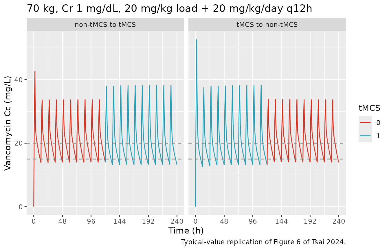
Figure 6 fully specifies one regimen: 70 kg, serum creatinine 1 mg/dL, a 20 mg/kg loading dose and 20 mg/kg/day maintenance given every 12 h. Infusions last 2 h (Methods, Simulation). The maintenance doses are taken to start one dosing interval after the load. The figure switches tMCS status at 120 h in both directions.

# One subject's event table: a loading dose, then maintenance every `tau` h
# from `tau` to `t_end`, 2-h infusions, and a dense observation grid on the
# central compartment. `mcs_switch` (h) flips MCS_TEMP_STATUS from `mcs` to
# 1 - mcs at that time.
make_regimen <- function(id, wt, creat, crrt, mcs, ld_mgkg, md_mgkg_day,
                         tau = 12, t_end = 240, mcs_switch = Inf, dt = 0.25) {
  dose_t <- c(0, seq(tau, t_end - tau, by = tau))
  dose_amt <- c(ld_mgkg * wt, rep(md_mgkg_day * wt * tau / 24, length(dose_t) - 1))
  keep <- dose_amt > 0
  doses <- data.frame(
    id = id, time = dose_t[keep], amt = dose_amt[keep], rate = dose_amt[keep] / 2,
    evid = 1L, cmt = "central"
  )
  obs <- data.frame(
    id = id, time = seq(0, t_end, by = dt), amt = 0, rate = 0,
    evid = 0L, cmt = "central"
  )
  ev <- dplyr::bind_rows(doses, obs) |> dplyr::arrange(time, dplyr::desc(evid))
  ev$WT <- wt
  ev$CREAT <- creat
  ev$RRT_CRRT_ACTIVE <- crrt
  ev$MCS_TEMP_STATUS <- ifelse(ev$time < mcs_switch, mcs, 1 - mcs)
  ev
}
mod_tv <- rxode2::zeroRe(mod)
#> ℹ parameter labels from comments will be replaced by 'label()'
solve_tv <- function(ev) {
  as.data.frame(rxode2::rxSolve(mod_tv, events = ev, rtol = 1e-10, atol = 1e-12, maxsteps = 1e6))
}

fig6_ev <- dplyr::bind_rows(
  make_regimen(1L, 70, 1, 0, mcs = 0, 20, 20, mcs_switch = 120) |>
    dplyr::mutate(panel = "non-tMCS to tMCS"),
  make_regimen(2L, 70, 1, 0, mcs = 1, 20, 20, mcs_switch = 120) |>
    dplyr::mutate(panel = "tMCS to non-tMCS")
)
fig6 <- as.data.frame(rxode2::rxSolve(
  mod_tv,
  events = fig6_ev, keep = c("panel", "MCS_TEMP_STATUS"),
  rtol = 1e-10, atol = 1e-12, maxsteps = 1e6
))
#> ℹ omega/sigma items treated as zero: 'etalcl', 'etalvp', 'etalq'
#> Warning: multi-subject simulation without without 'omega'
ggplot(fig6, aes(time, Cc, colour = factor(MCS_TEMP_STATUS), group = 1)) +
  geom_line() +
  geom_hline(yintercept = c(15, 20), linetype = "dashed", colour = "grey50") +
  facet_wrap(~panel) +
  scale_colour_manual(values = c("0" = "#d7301f", "1" = "#1f9eb4"), name = "tMCS") +
  scale_x_continuous(breaks = seq(0, 240, 48)) +
  labs(
    x = "Time (h)", y = "Vancomycin Cc (mg/L)",
    title = "70 kg, Cr 1 mg/dL, 20 mg/kg load + 20 mg/kg/day q12h",
    caption = "Typical-value replication of Figure 6 of Tsai 2024."
  )

# Rolling 24-h AUC of the typical subject on each side of the switch: the
# tMCS status changes Q only, so the daily AUC must not move.
auc24 <- function(sim, from) {
  s <- sim[sim$time >= from & sim$time <= from + 24, ]
  sum(diff(s$time) * (head(s$Cc, -1) + tail(s$Cc, -1)) / 2)
}
fig6_auc <- fig6 |>
  dplyr::group_by(panel) |>
  dplyr::group_modify(~ data.frame(
    window = c("96-120 h", "192-216 h"),
    auc24 = c(auc24(.x, 96), auc24(.x, 192))
  )) |>
  dplyr::ungroup()
knitr::kable(fig6_auc, digits = 1, caption = "Typical-value 24-h AUC (mg*h/L) before and after the tMCS switch.")

Typical-value 24-h AUC (mg*h/L) before and after the tMCS switch.

panel	window	auc24
non-tMCS to tMCS	96-120 h	491.2
non-tMCS to tMCS	192-216 h	491.2
tMCS to non-tMCS	96-120 h	491.1
tMCS to non-tMCS	192-216 h	491.3

# Daily dose / CL = 1400 / 2.85 = 491 mg*h/L once near steady state; the
# switch must leave it unchanged. The 0.5% bound is far above the trapezoid
# error at a 0.25-h grid and far below the 48% change in Q.
stopifnot(
  nrow(fig6_auc) == 4L,
  all(abs(fig6_auc$auc24 / (1400 / 2.85) - 1) < 0.02),
  abs(fig6_auc$auc24[1] / fig6_auc$auc24[2] - 1) < 0.005,
  abs(fig6_auc$auc24[3] / fig6_auc$auc24[4] - 1) < 0.005
)

The typical-value curves reproduce the shape of Figure 6: the tMCS segment has higher peaks and lower troughs at the same daily AUC (about 490 mg*h/L, the orange dashed line of the figure). The figure caption calls the tMCS line red and the non-tMCS line green, but the figure’s own legend (tMCS 0 red, 1 teal) and panel titles show the reverse; the colours above follow the legend.

Table 4 reports the population mean trough at 48 h for this regimen as 14.2 mg/L without and 13.4 mg/L with tMCS (also quoted in the Abstract, which prints the unit as mg/dL). The typical-value trough sits slightly below the population mean, as expected for a log-normally distributed clearance.

trough_tv <- function(wt, creat, crrt, mcs, ld, md, tau = 12) {
  s <- solve_tv(make_regimen(1L, wt, creat, crrt, mcs, ld, md, tau = tau, t_end = 60))
  s$Cc[s$time == 48]
}
row70 <- tibble::tibble(
  arm = c("non-tMCS", "tMCS"),
  paper_mean = c(14.2, 13.4),
  model_typical = c(trough_tv(70, 1, 0, 0, 20, 20), trough_tv(70, 1, 0, 1, 20, 20))
) |>
  dplyr::mutate(pct_diff = 100 * (model_typical / paper_mean - 1))
#> ℹ omega/sigma items treated as zero: 'etalcl', 'etalvp', 'etalq'
#> ℹ omega/sigma items treated as zero: 'etalcl', 'etalvp', 'etalq'
row70 |>
  dplyr::rename(
    "Arm" = arm, "Table 4 mean trough (mg/L)" = paper_mean,
    "Typical-value trough (mg/L)" = model_typical, "% diff" = pct_diff
  ) |>
  knitr::kable(digits = 2, caption = "48-h trough, 70 kg, Cr 1 mg/dL, 20 mg/kg load + 20 mg/kg/day q12h.")

48-h trough, 70 kg, Cr 1 mg/dL, 20 mg/kg load + 20 mg/kg/day q12h.

Arm	Table 4 mean trough (mg/L)	Typical-value trough (mg/L)	% diff
non-tMCS	14.2	13.95	-1.78
tMCS	13.4	13.14	-1.93

# Measured -1.8% / -1.9%. A mis-transcribed CL, Vc, Q or tMCS effect moves
# the trough by tens of percent; 5% leaves room for the mean-vs-typical gap.
stopifnot(
  all(abs(row70$pct_diff) < 5),
  # The tMCS-induced drop: paper 0.8 mg/L.
  abs(diff(rev(row70$model_typical)) - 0.8) < 0.15
)

Table 4: all scenarios

Table 4 lists the regimen with the best average probability of target attainment over the first 48 h for 15 scenarios (60, 70 and 80 kg crossed with creatinine 0.5, 1, 2 and 4 mg/dL or CRRT), with the mean 48-h trough under each tMCS status. The table does not state the dosing interval of each regimen (Figure 4 explores every 6, 8 or 12 h), so the absolute troughs below assume every 12 h and are shown for orientation only. The ratio of the tMCS to the non-tMCS trough is a property of the Q effect and is compared directly.

t4 <- tibble::tribble(
  ~wt, ~renal, ~ld, ~md, ~trough_tmcs, ~trough_non,
  60, "Cr=0.5", 25, 30, 13.4, 14.5,
  60, "Cr=1", 25, 20, 13.9, 14.7,
  60, "Cr=2", 15, 15, 17.6, 18.4,
  60, "Cr=4", 15, 10, 17.8, 18.4,
  60, "CRRT", 25, 15, 17.8, 17.6,
  70, "Cr=0.5", 25, 30, 10.8, 11.5,
  70, "Cr=1", 20, 20, 13.4, 14.2,
  70, "Cr=2", 15, 15, 17.1, 18.0,
  70, "Cr=4", 15, 10, 17.7, 18.3,
  70, "CRRT", 20, 15, 16.9, 17.5,
  80, "Cr=0.5", 20, 30, 12.1, 13.3,
  80, "Cr=1", 20, 20, 12.7, 13.5,
  80, "Cr=2", 15, 10, 15.3, 15.8,
  80, "Cr=4", 15, 10, 17.3, 18.0,
  80, "CRRT", 20, 15, 16.5, 17.1
) |>
  dplyr::mutate(
    crrt = as.integer(renal == "CRRT"),
    # CREAT does not enter the CRRT arm; any positive value is inert there.
    creat = ifelse(crrt == 1L, 1, suppressWarnings(as.numeric(sub("Cr=", "", renal))))
  )
stopifnot(nrow(t4) == 15L, !anyNA(t4$creat))
t4$model_tmcs <- mapply(trough_tv, t4$wt, t4$creat, t4$crrt, 1L, t4$ld, t4$md)
#> ℹ omega/sigma items treated as zero: 'etalcl', 'etalvp', 'etalq'
#> ℹ omega/sigma items treated as zero: 'etalcl', 'etalvp', 'etalq'
#> ℹ omega/sigma items treated as zero: 'etalcl', 'etalvp', 'etalq'
#> ℹ omega/sigma items treated as zero: 'etalcl', 'etalvp', 'etalq'
#> ℹ omega/sigma items treated as zero: 'etalcl', 'etalvp', 'etalq'
#> ℹ omega/sigma items treated as zero: 'etalcl', 'etalvp', 'etalq'
#> ℹ omega/sigma items treated as zero: 'etalcl', 'etalvp', 'etalq'
#> ℹ omega/sigma items treated as zero: 'etalcl', 'etalvp', 'etalq'
#> ℹ omega/sigma items treated as zero: 'etalcl', 'etalvp', 'etalq'
#> ℹ omega/sigma items treated as zero: 'etalcl', 'etalvp', 'etalq'
#> ℹ omega/sigma items treated as zero: 'etalcl', 'etalvp', 'etalq'
#> ℹ omega/sigma items treated as zero: 'etalcl', 'etalvp', 'etalq'
#> ℹ omega/sigma items treated as zero: 'etalcl', 'etalvp', 'etalq'
#> ℹ omega/sigma items treated as zero: 'etalcl', 'etalvp', 'etalq'
#> ℹ omega/sigma items treated as zero: 'etalcl', 'etalvp', 'etalq'
t4$model_non <- mapply(trough_tv, t4$wt, t4$creat, t4$crrt, 0L, t4$ld, t4$md)
#> ℹ omega/sigma items treated as zero: 'etalcl', 'etalvp', 'etalq'
#> ℹ omega/sigma items treated as zero: 'etalcl', 'etalvp', 'etalq'
#> ℹ omega/sigma items treated as zero: 'etalcl', 'etalvp', 'etalq'
#> ℹ omega/sigma items treated as zero: 'etalcl', 'etalvp', 'etalq'
#> ℹ omega/sigma items treated as zero: 'etalcl', 'etalvp', 'etalq'
#> ℹ omega/sigma items treated as zero: 'etalcl', 'etalvp', 'etalq'
#> ℹ omega/sigma items treated as zero: 'etalcl', 'etalvp', 'etalq'
#> ℹ omega/sigma items treated as zero: 'etalcl', 'etalvp', 'etalq'
#> ℹ omega/sigma items treated as zero: 'etalcl', 'etalvp', 'etalq'
#> ℹ omega/sigma items treated as zero: 'etalcl', 'etalvp', 'etalq'
#> ℹ omega/sigma items treated as zero: 'etalcl', 'etalvp', 'etalq'
#> ℹ omega/sigma items treated as zero: 'etalcl', 'etalvp', 'etalq'
#> ℹ omega/sigma items treated as zero: 'etalcl', 'etalvp', 'etalq'
#> ℹ omega/sigma items treated as zero: 'etalcl', 'etalvp', 'etalq'
#> ℹ omega/sigma items treated as zero: 'etalcl', 'etalvp', 'etalq'
t4 <- t4 |>
  dplyr::mutate(
    ratio_paper = trough_tmcs / trough_non,
    ratio_model = model_tmcs / model_non
  )
t4 |>
  dplyr::select(wt, renal, ld, md, trough_non, model_non, trough_tmcs, model_tmcs, ratio_paper, ratio_model) |>
  dplyr::rename(
    "BW (kg)" = wt, "Renal" = renal, "Load (mg/kg)" = ld, "Maint. (mg/kg/day)" = md,
    "Paper non-tMCS" = trough_non, "Model non-tMCS (q12h)" = model_non,
    "Paper tMCS" = trough_tmcs, "Model tMCS (q12h)" = model_tmcs,
    "Paper ratio" = ratio_paper, "Model ratio" = ratio_model
  ) |>
  knitr::kable(digits = 2, caption = "48-h trough (mg/L): Table 4 population means versus typical-value model troughs.")

48-h trough (mg/L): Table 4 population means versus typical-value model troughs.

BW (kg)	Renal	Load (mg/kg)	Maint. (mg/kg/day)	Paper non-tMCS	Model non-tMCS (q12h)	Paper tMCS	Model tMCS (q12h)	Paper ratio	Model ratio
60	Cr=0.5	25	30	14.5	10.56	13.4	9.87	0.92	0.93
60	Cr=1	25	20	14.7	14.28	13.9	13.52	0.95	0.95
60	Cr=2	15	15	18.4	17.14	17.6	16.36	0.96	0.95
60	Cr=4	15	10	18.4	18.75	17.8	18.13	0.97	0.97
60	CRRT	25	15	17.6	15.23	17.8	14.65	1.01	0.96
70	Cr=0.5	25	30	11.5	10.35	10.8	9.67	0.94	0.93
70	Cr=1	20	20	14.2	13.95	13.4	13.14	0.94	0.94
70	Cr=2	15	15	18.0	18.00	17.1	17.13	0.95	0.95
70	Cr=4	15	10	18.3	20.22	17.7	19.50	0.97	0.96
70	CRRT	20	15	17.5	14.84	16.9	14.22	0.97	0.96
80	Cr=0.5	20	30	13.3	10.04	12.1	9.35	0.91	0.93
80	Cr=1	20	20	13.5	14.00	12.7	13.17	0.94	0.94
80	Cr=2	15	10	15.8	13.62	15.3	12.98	0.97	0.95
80	Cr=4	15	10	18.0	21.45	17.3	20.64	0.96	0.96
80	CRRT	20	15	17.1	15.22	16.5	14.57	0.96	0.96

ratio_diff <- t4$ratio_model - t4$ratio_paper
summary(ratio_diff)
#>      Min.   1st Qu.    Median      Mean   3rd Qu.      Max. 
#> -0.049176 -0.006158 -0.001514 -0.003740  0.001168  0.021517
# The model ratio is 0.93-0.97 in every scenario. The paper's ratios,
# formed from means rounded to 0.1 mg/L, scatter around it (0.91-1.01); the
# 60 kg CRRT row, where the paper's tMCS mean is ABOVE the non-tMCS mean, is
# the outlier. Gate the centre, not the extremes.
stopifnot(
  abs(median(ratio_diff)) < 0.02,
  all(t4$ratio_model < 1)
)

The tMCS effect on the trough is reproduced across the table: the model lowers the 48-h trough by 3-7% under tMCS in every scenario, and the paper’s ratios centre on the same value. The absolute troughs agree closely where the q12h assumption is likely (creatinine 1 mg/dL), and fall below the paper’s means in scenarios whose optimal regimen probably used a shorter interval (creatinine 0.5 mg/dL, CRRT); this is a limitation of the transcribed table, not of the model.

Stochastic replication of the 70 kg, Cr 1 mg/dL scenario

Table 4 also reports, for the Figure 6 regimen, the mean +/- SD 48-h trough and the probability that the 24-h AUC lands in 400-600 mg*h/L averaged over the first 48 h. Two hundred virtual 70 kg patients per arm are simulated with between-subject variability and residual error.

rxode2::rxSetSeed(20241112)
n_per_arm <- 200L
stoch_ev <- dplyr::bind_rows(lapply(0:1, function(m) {
  dplyr::bind_rows(lapply(seq_len(n_per_arm), function(i) {
    make_regimen(m * n_per_arm + i, 70, 1, 0, mcs = m, 20, 20, t_end = 48, dt = 0.5)
  })) |>
    dplyr::mutate(arm = ifelse(m == 1L, "tMCS", "non-tMCS"))
}))
stopifnot(!anyDuplicated(unique(stoch_ev[, c("id", "time", "evid")])))
stoch <- as.data.frame(rxode2::rxSolve(mod, events = stoch_ev, keep = "arm", maxsteps = 1e6))
#> ℹ parameter labels from comments will be replaced by 'label()'

trough48 <- stoch |>
  dplyr::filter(time == 48) |>
  dplyr::group_by(arm) |>
  dplyr::summarise(mean_trough = mean(sim), sd_trough = sd(sim), .groups = "drop")

pta <- stoch |>
  dplyr::group_by(arm, id) |>
  dplyr::summarise(
    auc_0_24 = sum(diff(time[time <= 24]) * (head(ipredSim[time <= 24], -1) + tail(ipredSim[time <= 24], -1)) / 2),
    auc_24_48 = sum(diff(time[time >= 24]) * (head(ipredSim[time >= 24], -1) + tail(ipredSim[time >= 24], -1)) / 2),
    .groups = "drop"
  ) |>
  dplyr::group_by(arm) |>
  dplyr::summarise(
    pta_400_600 = 100 * mean(c(auc_0_24 >= 400 & auc_0_24 <= 600, auc_24_48 >= 400 & auc_24_48 <= 600)),
    pta_400 = 100 * mean(c(auc_0_24 >= 400, auc_24_48 >= 400)),
    .groups = "drop"
  )

stoch_tab <- dplyr::left_join(trough48, pta, by = "arm") |>
  dplyr::mutate(
    paper_mean = c(14.2, 13.4)[match(arm, c("non-tMCS", "tMCS"))],
    paper_sd = c(3.0, 2.8)[match(arm, c("non-tMCS", "tMCS"))],
    paper_pta = c(62.2, 61.8)[match(arm, c("non-tMCS", "tMCS"))],
    paper_pta400 = c(78.9, 78.7)[match(arm, c("non-tMCS", "tMCS"))]
  )
stoch_tab |>
  dplyr::select(arm, paper_mean, mean_trough, paper_sd, sd_trough, paper_pta, pta_400_600, paper_pta400, pta_400) |>
  dplyr::rename(
    "Arm" = arm,
    "Trough mean, paper" = paper_mean, "Trough mean, model" = mean_trough,
    "Trough SD, paper" = paper_sd, "Trough SD, model" = sd_trough,
    "PTA 400-600 %, paper" = paper_pta, "PTA 400-600 %, model" = pta_400_600,
    "AUC >= 400 %, paper" = paper_pta400, "AUC >= 400 %, model" = pta_400
  ) |>
  knitr::kable(digits = 1, caption = "70 kg, Cr 1 mg/dL, 20 mg/kg load + 20 mg/kg/day q12h: 200 virtual patients per arm.")

70 kg, Cr 1 mg/dL, 20 mg/kg load + 20 mg/kg/day q12h: 200 virtual patients per arm.

Arm	Trough mean, paper	Trough mean, model	Trough SD, paper	Trough SD, model	PTA 400-600 %, paper	PTA 400-600 %, model	AUC >= 400 %, paper	AUC >= 400 %, model
non-tMCS	14.2	14.5	3.0	6.5	62.2	59.0	78.9	78.5
tMCS	13.4	13.6	2.8	6.1	61.8	60.8	78.7	77.5

# Mean trough: SD of the mean ~0.4 mg/L at n = 200 (~3%); 12% is several
# standard errors away from the measured ~1-4% gap and still fails on a
# structural transcription error.
stopifnot(
  nrow(stoch_tab) == 2L,
  all(abs(stoch_tab$mean_trough / stoch_tab$paper_mean - 1) < 0.12)
)

stoch |>
  dplyr::group_by(arm, time) |>
  dplyr::summarise(
    p05 = quantile(sim, 0.05), p50 = quantile(sim, 0.5), p95 = quantile(sim, 0.95),
    .groups = "drop"
  ) |>
  ggplot(aes(time, p50)) +
  geom_ribbon(aes(ymin = p05, ymax = p95), alpha = 0.25) +
  geom_line() +
  facet_wrap(~arm) +
  labs(
    x = "Time (h)", y = "Vancomycin Cc (mg/L)",
    title = "Median and 90% prediction interval, first 48 h",
    caption = "200 virtual 70 kg patients per arm, Cr 1 mg/dL, 20 mg/kg load + 20 mg/kg/day q12h."
  )

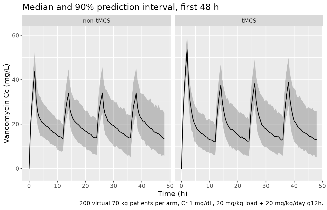
The mean trough and the AUC-based target attainment agree with Table 4, and the model reproduces the paper’s finding that the AUC-based PTA is unchanged by tMCS while the trough falls. The model’s trough SD is wider than the roughly 3 mg/L printed in Table 4. With a 32% CV on clearance and an additive 1.39 mg/L residual, a between-patient SD near 3 mg/L at a 14 mg/L mean is not attainable, so the printed SD may describe a different spread than the between-patient one (for example, without between-subject variability); the paper does not say.

PKNCA: index-dose NCA against Supplementary Table S2

Supplementary Table S2 gives the observed non-compartmental analysis of the sampled index dose stratified by tMCS. The virtual cohort below mirrors the index-dose design: 900 mg infused over 1.8 h every 12 h, the seventh dose sampled pre-dose and at 0.5, 1, 2, 3, 6, 9 and 12 h after the end of infusion, with no further dose inside that window. Weight and creatinine are drawn log-normally around the Table 1 medians, and the CRRT fraction per arm follows Table S2. The observed medians come from only 11 and 14 patients with heterogeneous dosing histories, so the comparison is approximate.

rxode2::rxSetSeed(2617)
set.seed(2617)
make_index_arm <- function(n, mcs, frac_crrt, id_offset) {
  subj <- tibble::tibble(
    id = id_offset + seq_len(n),
    WT = exp(rnorm(n, log(68.8), 0.2)),
    CREAT = exp(rnorm(n, log(1.1), 0.5)),
    RRT_CRRT_ACTIVE = rbinom(n, 1, frac_crrt),
    MCS_TEMP_STATUS = mcs,
    arm = ifelse(mcs == 1L, "tMCS", "non-tMCS")
  )
  dose_t <- seq(0, 72, by = 12)
  doses <- tidyr::expand_grid(subj, time = dose_t) |>
    dplyr::mutate(amt = 900, rate = 900 / 1.8, evid = 1L, cmt = "central")
  obs_t <- c(72, 72 + 1.8 + c(0.5, 1, 2, 3, 6, 9, 12))
  obs <- tidyr::expand_grid(subj, time = obs_t) |>
    dplyr::mutate(amt = 0, rate = 0, evid = 0L, cmt = "central")
  dplyr::bind_rows(doses, obs) |> dplyr::arrange(id, time, dplyr::desc(evid))
}
idx_ev <- dplyr::bind_rows(
  make_index_arm(200L, 1L, 2 / 11, 0L),
  make_index_arm(200L, 0L, 5 / 14, 200L)
)
stopifnot(!anyDuplicated(unique(idx_ev[, c("id", "time", "evid")])))
idx_sim <- as.data.frame(rxode2::rxSolve(mod, events = idx_ev, keep = "arm", maxsteps = 1e6))

conc_df <- idx_sim |>
  dplyr::filter(!is.na(Cc)) |>
  dplyr::select(id, time, Cc, arm)
dose_df <- idx_ev |>
  dplyr::filter(evid == 1L) |>
  dplyr::select(id, time, amt, arm)
conc_obj <- PKNCA::PKNCAconc(conc_df, Cc ~ time | arm + id)
dose_obj <- PKNCA::PKNCAdose(dose_df, amt ~ time | arm + id)
# CL_obs and Vd_obs are taken as dose / AUC0-inf and CL / lambda-z of the
# index dose, extrapolated from concentrations that still carry the earlier
# doses -- the naive single-dose NCA that a sampled index dose yields.
intervals <- data.frame(
  start = 72, end = Inf,
  cmax = TRUE, tmax = TRUE, aucinf.obs = TRUE, cl.obs = TRUE, vz.obs = TRUE,
  half.life = TRUE
)
nca_res <- PKNCA::pk.nca(PKNCA::PKNCAdata(conc_obj, dose_obj, intervals = intervals))

published <- tibble::tribble(
  ~arm, ~cmax, ~cl.obs, ~vz.obs, ~half.life,
  "tMCS", 26.5, 1.6, 35.6, 12.6,
  "non-tMCS", 41.6, 1.3, 24.2, 11.6
)
cmp <- nlmixr2lib::ncaComparisonTable(
  simulated = nca_res,
  reference = published,
  by = "arm",
  params = c("cmax", "half.life", "cl.obs", "vz.obs"),
  units = c(cmax = "mg/L", cl.obs = "L/h", vz.obs = "L", half.life = "h"),
  tolerance_pct = 20
)
# The comparison is IV: relabel PKNCA's generic CL/F and Vz/F.
cmp[[1]] <- sub("CL/F", "CL_obs = dose / AUC0-inf", cmp[[1]], fixed = TRUE)
cmp[[1]] <- sub("Vz/F", "Vd_obs = CL_obs / lambda-z", cmp[[1]], fixed = TRUE)
knitr::kable(
  cmp,
  caption = "Index-dose NCA: median of the virtual cohort versus the observed medians of Supplementary Table S2. * differs by >20%."
)

Index-dose NCA: median of the virtual cohort versus the observed medians of Supplementary Table S2. * differs by >20%.

NCA parameter	arm	Reference	Simulated	% diff
Cmax (mg/L)	tMCS	26.5	43.7	+64.8%*
Cmax (mg/L)	non-tMCS	41.6	37.8	-9.1%
t½ (h)	tMCS	12.6	16	+27.1%*
t½ (h)	non-tMCS	11.6	14.3	+23.4%*
CL_obs = dose / AUC0-inf (L/h)	tMCS	1.6	1.15	-27.9%*
CL_obs = dose / AUC0-inf (L/h)	non-tMCS	1.3	1.29	-0.9%
Vd_obs = CL_obs / lambda-z (L)	tMCS	35.6	25.2	-29.2%*
Vd_obs = CL_obs / lambda-z (L)	non-tMCS	24.2	24.6	+1.5%

The supplement does not define CL_obs and Vd_obs. Read as the naive single-dose NCA of the sampled dose (dose over an AUC0-inf that is extrapolated from concentrations still carrying the earlier doses, and Vd_obs as CL_obs over the terminal slope), the non-tMCS arm is reproduced closely: clearance, volume and peak all fall within 10% of the observed medians. Read instead as dose over the 12-h AUC, simulated clearance would be about twice the observed value, so this reading is the one the data support. The simulated half-life runs about 25% above both observed medians, whose interquartile ranges (8.4-44.7 h and 10.8-16.2 h) are wide.

The tMCS arm is not reproduced: the observed tMCS peak (26.5 mg/L) is lower than the non-tMCS one and the observed volume larger. The final model cannot produce that pattern for any patient. tMCS lowers Q only, which raises the post-infusion peak and leaves the volumes unchanged. The authors’ covariate search tested the presence, mode and flow of tMCS and retained only its effect on Q (Methods; Supplementary Table S3), so the observed tMCS medians reflect differences between these 11 patients that the final model does not attribute to tMCS. Two further cautions apply:

• The observed medians come from 11 and 14 patients whose earlier doses, amounts and creatinine trajectories varied, while the virtual cohort uses one fixed 900 mg q12h history.
• Table S2’s group sizes (11 tMCS, 14 non-tMCS) are the reverse of Table 1’s index-dose counts (14 on tMCS, 11 without), and its CRRT total (7) matches Table 1’s first-dose count rather than its index-dose count (6). The values are used as printed.

Assumptions and deviations

• Residual error scale. Table 2 prints the additive residual as 1.39 without stating whether it is a standard deviation or a variance. The model was fit in Phoenix NLME 8.2, whose residual-error estimate is a standard deviation, so addSd = 1.39 mg/L is used. Read as a variance it would be 1.18 mg/L.
• Which clearance arm carries creatinine. The Results prose says “an independent CL for non-CRRT with BW as a covariate and an independent CL for CRRT with serum Cr and BW as covariates”, which puts creatinine on the CRRT arm. The printed equation in Table 2, Supplementary Table S1 (Model 3: “Cr as a covariate only on CL for non-dialysis”) and the Discussion (“Cr level on decreasing the CL for non-CRRT”) all put it on the non-CRRT arm, and that reading is used.
• Creatinine is uncentred. CL = theta3 * Cr^theta5 * (BW/70)^theta6 takes creatinine in mg/dL with no reference value, so theta3 is the clearance at 1 mg/dL. CREAT must be a positive number on every record, including CRRT records where it has no effect.
• tMCS covariate. The paper’s tMCS pools VA-ECMO, VV-ECMO and extracorporeal VAD (2 of the 14 supported patients were on a CentriMag VAD, not ECMO), so it does not map onto ECMO_STATUS. The maintainers registered the broader canonical MCS_TEMP_STATUS for it.
• CRRT covariate. CRRT changed within the vancomycin course for one patient, so it is encoded with the time-varying gate RRT_CRRT_ACTIVE.
• Table 4 dosing interval. Table 4 does not give the interval of its recommended regimens; the troughs above assume every 12 h, which Figure 6 states for the 70 kg, Cr 1 mg/dL regimen. Maintenance doses are assumed to start one interval after the loading dose.
• Table 4 trough SD. The model’s between-patient spread of the 48-h trough is wider than the roughly 3 mg/L SD printed in Table 4; see the stochastic section above.
• Figure 6 colours. The caption labels the colours the opposite way from the figure’s legend and panel titles; the legend is followed.
• No erratum to Tsai 2024 was found as of 2026-10-15.