Tacrolimus (Zavrelova 2025)
Source:vignettes/articles/Zavrelova_2025_tacrolimus.Rmd
Zavrelova_2025_tacrolimus.RmdModel and source
- Citation: Zavrelova A, Zibridova K, Radocha J, Cermakova E, Rozsivalova P, Zak P, Visek B, Lanska M, Stevkova J, Merdita S, Slanar O, Sima M. Tacrolimus exposure during the three-month period following allogeneic stem cell transplantation predicts overall survival. Front Pharmacol. 2025;16:1517083. doi:10.3389/fphar.2025.1517083
- Description: One-compartment population PK model for continuous-infusion intravenous tacrolimus (whole blood) in adults after allogeneic haematopoietic stem cell transplantation (Zavrelova 2025); clearance declines exponentially with age and is 23% lower in a repeat transplantation, and volume of distribution carries no covariate
- Article: https://doi.org/10.3389/fphar.2025.1517083
Zavrelova 2025 related tacrolimus exposure over the first three months after allogeneic haematopoietic stem cell transplantation to overall survival, and developed a one-compartment population PK model for the initial continuous intravenous infusion phase so that a maximum starting dose could be proposed. Tacrolimus clearance declines exponentially with age and is 23% lower in a repeat transplantation; the volume of distribution (127.1 L) carries no covariate. From the model the authors derived a nomogram (Figure 2) giving the maximum initial daily intravenous dose that keeps exposure below the first-month survival cutoff of 279 ng.h/mL.
Population
The PK analysis pooled 349 whole-blood tacrolimus concentrations (2-7 per case) from 100 allogeneic peripheral blood stem cell transplantations performed at University Hospital Hradec Kralove, Czech Republic, in 2016-2018: 86 first transplantations and 14 repeat transplantations (Results 3.5). Only concentrations from the initial continuous intravenous infusion were modelled. Table 1 of the source describes the 86 first-transplant patients: 41.9% female, median age 58 years (range 20-72), median weight 82 kg (range 49-133), median BSA 1.96 m^2. Most were transplanted for AML (50%), MDS (14%), ALL (9.3%) or CLL / lymphoma (12.8%); 59.3% had high-risk disease and 59.3% received myeloablative conditioning. All patients were white and all received mycophenolate mofetil, rabbit anti-thymocyte globulin and an azole antifungal.
Tacrolimus was started at 0.03 mg/kg as a continuous intravenous infusion on the day before transplantation and switched to oral dosing around day 11, with dose adjustment to a 5-15 ng/mL target and for voriconazole or posaconazole co-administration (Methods 2.1).
The same information is available programmatically via the model’s
population metadata
(rxode2::rxode(readModelDb("Zavrelova_2025_tacrolimus"))$population).
Source trace
The per-parameter origin is recorded as an in-file comment next to
each ini() entry in
inst/modeldb/specificDrugs/Zavrelova_2025_tacrolimus.R. The
table below collects them in one place.
| Equation / parameter | Value | Source location |
|---|---|---|
| One compartment, linear elimination, combined residual error | n/a | Results 3.5, second paragraph |
Vd = Vd_pop |
n/a | Results 3.5, printed covariate equations |
CL = CL_pop * exp(beta_CL_age * age) * exp(beta_CL_repeated Tx [if yes]) |
n/a | Results 3.5, printed covariate equations |
CL = 7.94 * exp(-0.0085 * age) * exp(-0.26 [if repeated Tx]) |
n/a | Results 3.5; Abstract |
lvc (Vd_pop) |
127.1 L | Table 4 (RSE 7.9%) |
lcl (CL_pop) |
7.94 L/h | Table 4 (RSE 15.3%) |
e_age_cl (beta_CL_age) |
-0.0085 /year | Table 4 (RSE 32.2%) |
e_hctprior_cl (beta_CL_repeated Tx) |
-0.26 | Table 4 (RSE 37.2%) |
etalvc (Omega_Vd) |
0.45 SD -> 0.2025 var | Table 4 (RSE 18.6%) |
etalcl (Omega_CL) |
0.29 SD -> 0.0841 var | Table 4 (RSE 8.6%) |
addSd (Constant) |
0.0018 mg/L = 1.8 ng/mL | Table 4 (RSE 15.6%) |
propSd (Proportional) |
0.17 | Table 4 (RSE 11.2%) |
AGE covariate, uncentred |
median 58 y | Table 1; Results 3.5 worked example (57 y) |
HCT_PRIOR covariate |
repeat vs first transplantation | Results 3.5; Table 4 |
| Typical CL 4.89 L/h (57 y, first Tx) and 3.77 L/h (repeat Tx) | n/a | Results 3.5 |
| Nomogram: dose = CL x 279 ng.h/mL | n/a | Discussion; Figure 2 |
| AUCtc cutoffs 279 / 258 / 160 / 222 ng.h/mL | n/a | Results 3.2; Table 2; Supplementary ROC reports |
Typical-value replication
Results 3.5 gives two worked typical values: “in a 57-year-old patient (the median age in our population), who undergoes his/her first transplantation, the estimated tacrolimus clearance is 4.89 L/h”, and 3.77 L/h for the same patient in a repeat transplantation.
mod <- readModelDb("Zavrelova_2025_tacrolimus")
ui <- rxode2::rxode(mod)
#> ℹ parameter labels from comments will be replaced by 'label()'
mod_typical <- rxode2::zeroRe(ui)

typical_cl <- function(age, hct_prior) {
  ev <- data.frame(
    id = 1L, time = c(0, 1), amt = c(1, NA_real_), rate = c(NA_real_, NA_real_),
    evid = c(1L, 0L), cmt = "central", AGE = age, HCT_PRIOR = hct_prior
  )
  s <- rxode2::rxSolve(mod_typical, ev, returnType = "data.frame")
  c(cl = s$cl[1], vc = s$vc[1])
}

first <- typical_cl(57, 0)
#> ℹ omega/sigma items treated as zero: 'etalvc', 'etalcl'
repeat_tx <- typical_cl(57, 1)
#> ℹ omega/sigma items treated as zero: 'etalvc', 'etalcl'

typical_cmp <- tibble::tibble(
  quantity = c("CL, first transplantation (L/h)", "CL, repeat transplantation (L/h)",
               "CL repeat / first (fraction)", "Vd (L)"),
  model = c(first[["cl"]], repeat_tx[["cl"]], repeat_tx[["cl"]] / first[["cl"]], first[["vc"]]),
  published = c(4.89, 3.77, 0.77, 127.1)
) |>
  mutate(difference_pct = 100 * (model - published) / published)

typical_cmp |>
  rename("Quantity" = quantity, "Model" = model, "Published" = published,
         "Difference (%)" = difference_pct) |>
  knitr::kable(digits = 3,
caption = "Typical values for a 57-year-old patient against Results 3.5 of Zavrelova 2025.")| Quantity | Model | Published | Difference (%) |
|---|---|---|---|
| CL, first transplantation (L/h) | 4.891 | 4.89 | 0.022 |
| CL, repeat transplantation (L/h) | 3.771 | 3.77 | 0.034 |
| CL repeat / first (fraction) | 0.771 | 0.77 | 0.137 |
| Vd (L) | 127.100 | 127.10 | 0.000 |
# Deterministic: the paper quotes these to 3 significant figures, so the model
# must reproduce them to within that rounding.
stopifnot(
  abs(first[["cl"]] - 4.89) < 0.005,
  abs(repeat_tx[["cl"]] - 3.77) < 0.005,
  abs(repeat_tx[["cl"]] / first[["cl"]] - 0.77) < 0.005,
  abs(first[["vc"]] - 127.1) < 1e-6
)
The typical elimination half-life at 57 years is 18.0 h for a first transplantation and 23.4 h for a repeat transplantation.
Exposure arithmetic
The survival analysis expresses exposure as the area under the curve
of trough concentrations (AUCtc), normalised per 24 h, so a constant
concentration C corresponds to AUCtc = 24 * C.
The Discussion and Conclusion convert the ROC cutoffs into trough
concentrations with that identity.
cutoffs <- tibble::tribble(
  ~period,                ~auctc, ~trough_discussion, ~trough_abstract,
  "First month",           279,   11.6,               NA,
  "Second month",          258,   10.8,               10.7,
  "Third month",           160,    6.7,                6.8,
  "Whole 3-month period",  222,     NA,                NA
) |>
  mutate(trough_identity = auctc / 24)

cutoffs |>
  rename("Period" = period, "AUCtc cutoff (ng.h/mL)" = auctc,
         "Trough, Discussion (ng/mL)" = trough_discussion,
         "Trough, Abstract (ng/mL)" = trough_abstract,
         "AUCtc / 24 (ng/mL)" = trough_identity) |>
  knitr::kable(digits = 2,
caption = "ROC-derived AUCtc cutoffs (Results 3.2) and their trough-concentration equivalents as quoted in the Discussion / Conclusion and in the Abstract.")| Period | AUCtc cutoff (ng.h/mL) | Trough, Discussion (ng/mL) | Trough, Abstract (ng/mL) | AUCtc / 24 (ng/mL) |
|---|---|---|---|---|
| First month | 279 | 11.6 | NA | 11.62 |
| Second month | 258 | 10.8 | 10.7 | 10.75 |
| Third month | 160 | 6.7 | 6.8 | 6.67 |
| Whole 3-month period | 222 | NA | NA | 9.25 |
chk <- cutoffs |> filter(!is.na(trough_discussion))
stopifnot(nrow(chk) == 3L, all(abs(chk$trough_identity - chk$trough_discussion) < 0.06))
The Discussion values (11.6, 10.8, 6.7 ng/mL) are the identity rounded to one decimal. The Abstract quotes 10.7 and 6.8 ng/mL for the second and third months, which differ from the identity by one rounding unit in opposite directions.
Replicate Figure 2 (dosing nomogram)
The nomogram gives the maximum initial daily intravenous dose in a
first transplantation as dose = CL x AUC, with the typical
clearance at each age and the first-month cutoff of 279 ng.h/mL. The
chunk below doses each age with that daily amount as a continuous
infusion, solves the typical-value model to steady state, and checks
that 24 * Css returns 279 ng.h/mL. The two curve end points
read from Figure 2 (about 1.87 mg at 20 years and 1.20 mg at 72 years)
are checked against the closed form.
auc_cut <- 279 # ng.h/mL, first-month AUCtc cutoff
ages_nomo <- seq(20, 72, by = 4)
cl_typ <- 7.94 * exp(-0.0085 * ages_nomo)
dose_day <- cl_typ * auc_cut / 1000 # L/h x ng.h/mL / 1000 = mg per 24 h

t_end_nomo <- 480 # >= 20 typical half-lives at every age
nomo_ev <- bind_rows(
  tibble::tibble(id = seq_along(ages_nomo), time = 0,
                 amt = dose_day * t_end_nomo / 24, rate = dose_day / 24, evid = 1L),
  tidyr::expand_grid(id = seq_along(ages_nomo), time = c(0, t_end_nomo)) |>
    mutate(amt = NA_real_, rate = NA_real_, evid = 0L)
) |>
  mutate(cmt = "central", AGE = ages_nomo[id], HCT_PRIOR = 0L) |>
  arrange(id, time, desc(evid))

nomo_sim <- rxode2::rxSolve(mod_typical, nomo_ev, returnType = "data.frame",
                            rtol = 1e-10, atol = 1e-12) |>
  filter(time == t_end_nomo) |>
  mutate(AGE = ages_nomo[id], dose_day = dose_day[id], auc24 = 24 * Cc)
#> ℹ omega/sigma items treated as zero: 'etalvc', 'etalcl'
#> Warning: multi-subject simulation without without 'omega'

# Same drawn (typical) parameters on both sides: pure numerical error.
stopifnot(nrow(nomo_sim) == length(ages_nomo),
          max(abs(nomo_sim$auc24 / auc_cut - 1)) < 1e-4)

fig2_points <- tibble::tibble(AGE = c(20, 72), dose_fig = c(1.87, 1.20))
fig2_cmp <- fig2_points |>
  mutate(dose_model = 7.94 * exp(-0.0085 * AGE) * auc_cut / 1000)
stopifnot(all(abs(fig2_cmp$dose_model - fig2_cmp$dose_fig) < 0.02))

fig2_cmp |>
  rename("Age (years)" = AGE, "Figure 2, read (mg/day)" = dose_fig,
         "Model (mg/day)" = dose_model) |>
knitr::kable(digits = 3, caption = "Nomogram end points read from Figure 2 against the model's typical CL x 279 ng.h/mL.")| Age (years) | Figure 2, read (mg/day) | Model (mg/day) |
|---|---|---|
| 20 | 1.87 | 1.869 |
| 72 | 1.20 | 1.201 |
ggplot(nomo_sim, aes(AGE, dose_day)) +
  geom_line(linewidth = 1) +
  geom_point(data = fig2_points, aes(AGE, dose_fig), colour = "firebrick", size = 3) +
  scale_y_continuous(limits = c(1, 2)) +
  labs(x = "Age (years)", y = "Tacrolimus daily dose (mg)",
       caption = paste("Replicates Figure 2 of Zavrelova 2025. Line = typical CL(age) x 279 ng.h/mL;",
                       "red points = end points read from the published figure.")) +
  theme_bw()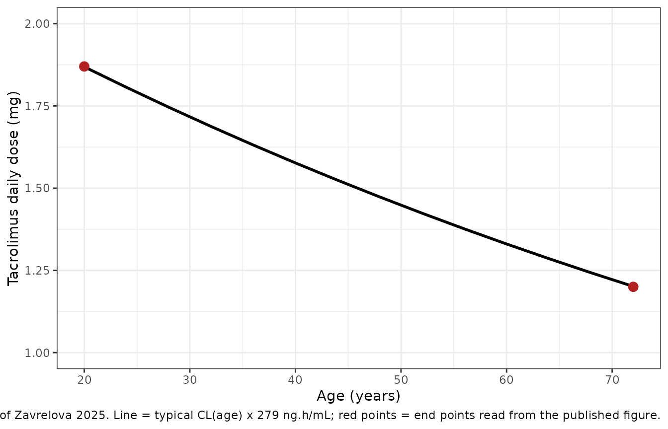
The repeat-transplantation dose is lower by the same factor as clearance, exp(-0.26) = 0.77, which the Discussion states as “further reduced by 23%”.
Virtual cohort
Observed data are not available. The cohort below approximates Table 1: age drawn from a normal distribution around the median of 58 years (SD 11) truncated to the 20-72-year range, weight from a log-normal distribution around 82 kg (log-SD 0.2) truncated to 49-133 kg, and 14% repeat transplantations (14 of the 100 transplantations in the PK dataset). Every subject receives the protocol starting dose, 0.03 mg/kg/day by continuous intravenous infusion, for 11 days (264 h), which is the intravenous phase the model was fitted to. The simulation uses no dose adjustment, so it shows what the starting dose alone would produce rather than the TDM-adjusted concentrations of the source.
set.seed(20250509)
n_sub <- 200L

draw_trunc <- function(n, draw, lo, hi) {
  x <- numeric(0)
  while (length(x) < n) {
    cand <- draw(2 * n)
    x <- c(x, cand[cand >= lo & cand <= hi])
  }
  x[seq_len(n)]
}

cohort <- tibble::tibble(
  id = seq_len(n_sub),
  AGE = draw_trunc(n_sub, function(n) rnorm(n, 58, 11), 20, 72),
  WT = draw_trunc(n_sub, function(n) 82 * exp(rnorm(n, 0, 0.2)), 49, 133),
  HCT_PRIOR = as.integer(seq_len(n_sub) <= round(0.14 * n_sub))
)

t_iv <- 264 # 11 days of continuous infusion
obs_times <- seq(0, t_iv, by = 1)
rate_mg_h <- 0.03 * cohort$WT / 24

events <- bind_rows(
  cohort |> transmute(id, time = 0, amt = rate_mg_h * t_iv, rate = rate_mg_h, evid = 1L),
  tidyr::expand_grid(id = cohort$id, time = obs_times) |>
    mutate(amt = NA_real_, rate = NA_real_, evid = 0L)
) |>
  left_join(cohort |> select(id, AGE, HCT_PRIOR), by = "id") |>
  mutate(cmt = "central", treatment = "0.03 mg/kg/day CIV") |>
  arrange(id, time, desc(evid))

stopifnot(n_distinct(events$id) == n_sub, sum(events$evid == 1L) == n_sub)
Simulation
rxode2::rxSetSeed(20250509)
sim <- rxode2::rxSolve(mod, events = events, keep = c("treatment"),
                       returnType = "data.frame")
#> ℹ parameter labels from comments will be replaced by 'label()'
if (is.null(sim$id)) sim$id <- 1L

stopifnot(nrow(sim) == n_sub * length(obs_times), !anyNA(sim$Cc),
          all(sim$Cc >= -1e-6 * max(sim$Cc)))
Cc is the individual prediction; the residual error is
not applied.
bands <- sim |>
  group_by(time) |>
  summarise(p05 = quantile(Cc, 0.05), p50 = median(Cc), p95 = quantile(Cc, 0.95),
            .groups = "drop")

ggplot(bands, aes(time / 24, p50)) +
  geom_ribbon(aes(ymin = p05, ymax = p95), fill = "steelblue", alpha = 0.3) +
  geom_line(linewidth = 0.8) +
  geom_hline(yintercept = c(5, 15), linetype = "dashed", colour = "grey40") +
  geom_hline(yintercept = auc_cut / 24, linetype = "dotted", colour = "firebrick") +
  labs(x = "Time since start of infusion (days)", y = "Tacrolimus whole blood (ng/mL)",
       caption = paste("Median and 5th-95th percentiles, 200 virtual patients on 0.03 mg/kg/day",
                       "continuous infusion with no TDM adjustment. Dashed: 5-15 ng/mL target range;",
                       "dotted: 11.6 ng/mL, the first-month cutoff (279 ng.h/mL / 24).")) +
  theme_bw()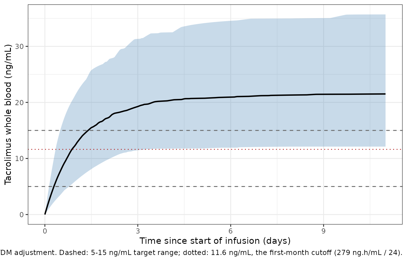
At the protocol starting dose most virtual patients rise above both the 15 ng/mL target ceiling and the first-month survival cutoff. The source reports a median trough of 10 ng/mL by day 10 under routine TDM (Discussion), which implies that the starting dose was reduced in most patients; the nomogram’s typical maximum of about 1.4 mg/day at 57 years is roughly half of the 2.5 mg/day that 0.03 mg/kg gives at the median weight of 82 kg.
day11 <- sim |> filter(time == t_iv)
cat(sprintf("Median day-11 concentration at 0.03 mg/kg/day: %.1f ng/mL\n", median(day11$Cc)))
#> Median day-11 concentration at 0.03 mg/kg/day: 21.5 ng/mL
# Typical-value Css for the median patient: 0.03 * 82 mg/day / (24 * CL(58)) -> ng/mL.
css_typ <- 1000 * 0.03 * 82 / (24 * 7.94 * exp(-0.0085 * 58))
cat(sprintf("Typical steady state for an 82-kg, 58-year-old patient: %.1f ng/mL\n", css_typ))
#> Typical steady state for an 82-kg, 58-year-old patient: 21.1 ng/mL
# Structural: a wrong CL, dose or unit moves the cohort median by tens of percent.
# The cohort median sits near the typical value because CL is log-normal (so the
# median of 1/CL is 1/median CL); the slowest subjects are not yet at steady
# state on day 11, which pulls the median down by a few percent at most.
stopifnot(median(day11$Cc) > 0.8 * css_typ, median(day11$Cc) < 1.25 * css_typ)
PKNCA validation
The source reports no NCA results for its data, so there is nothing
to put in a side-by-side comparison table. PKNCA is instead checked
against an exact per-subject mass-balance identity: for an intravenous
infusion with linear elimination,
CL * AUC(0, t) = amount infused by t - amount remaining at t.
conc_df <- sim |>
  filter(!is.na(Cc)) |>
  mutate(Cc = pmax(Cc, 0)) |>
  select(id, time, Cc, treatment)

dose_df <- events |>
  filter(evid == 1L) |>
  mutate(duration = amt / rate) |>
  select(id, time, amt, duration, treatment)

conc_obj <- PKNCA::PKNCAconc(conc_df, Cc ~ time | treatment / id)
dose_obj <- PKNCA::PKNCAdose(dose_df, amt ~ time | treatment + id,
                             route = "intravascular", duration = "duration")

intervals <- data.frame(
  start = c(0, 240), end = c(t_iv, t_iv),
  auclast = c(TRUE, FALSE), cmax = c(FALSE, TRUE), cmin = c(FALSE, TRUE),
  cav = c(FALSE, TRUE)
)

nca_res <- PKNCA::pk.nca(PKNCA::PKNCAdata(conc_obj, dose_obj, intervals = intervals,
                                          options = list(auc.method = "linear")))

nca_tab <- as.data.frame(nca_res) |>
  mutate(interval = paste0(start, "-", end, " h")) |>
  group_by(treatment, interval, PPTESTCD) |>
  summarise(median = median(PPORRES), p05 = quantile(PPORRES, 0.05),
            p95 = quantile(PPORRES, 0.95), .groups = "drop")

nca_tab |>
  rename("Treatment" = treatment, "Interval" = interval, "Parameter" = PPTESTCD,
         "Median" = median, "5th percentile" = p05, "95th percentile" = p95) |>
knitr::kable(digits = 1, caption = "PKNCA summary of the virtual cohort (ng/mL; ng.h/mL for AUC).")| Treatment | Interval | Parameter | Median | 5th percentile | 95th percentile |
|---|---|---|---|---|---|
| 0.03 mg/kg/day CIV | 0-264 h | auclast | 5072.5 | 2899.7 | 8186.9 |
| 0.03 mg/kg/day CIV | 240-264 h | auclast | 515.8 | 290.8 | 856.6 |
| 0.03 mg/kg/day CIV | 240-264 h | cav | 21.5 | 12.1 | 35.7 |
| 0.03 mg/kg/day CIV | 240-264 h | cmax | 21.5 | 12.1 | 35.7 |
| 0.03 mg/kg/day CIV | 240-264 h | cmin | 21.5 | 12.1 | 35.7 |
auc_0t <- as.data.frame(nca_res) |>
  filter(PPTESTCD == "auclast", start == 0) |>
  select(id, auclast = PPORRES)

end_state <- sim |>
  filter(time == t_iv) |>
  select(id, central, cl) |>
  left_join(cohort |> select(id, WT), by = "id") |>
  mutate(infused = 0.03 * WT / 24 * t_iv,
         auc_mass_balance = 1000 * (infused - central) / cl) # mg.h/L -> ng.h/mL

mb <- inner_join(auc_0t, end_state, by = "id") |>
  mutate(pct_diff = 100 * (auclast - auc_mass_balance) / auc_mass_balance)

cat(sprintf("PKNCA AUC0-264 vs mass balance: median |diff| %.4f%%, max |diff| %.4f%%\n",
            median(abs(mb$pct_diff)), max(abs(mb$pct_diff))))
#> PKNCA AUC0-264 vs mass balance: median |diff| 0.0014%, max |diff| 0.0033%

# Both sides use the same drawn parameters, so the difference is only the
# linear-trapezoid error of a 1-h grid on a smooth rising curve plus ODE
# tolerance; a wrong unit or a dropped dose moves it by orders of magnitude.
stopifnot(nrow(mb) == n_sub, max(abs(mb$pct_diff)) < 0.5)
Assumptions and deviations
-
Unit of the additive residual error. Table 4 prints
the constant error term as 0.0018 with no unit. With doses in mg and
volume in L the model predicts in mg/L, so 0.0018 is read as mg/L,
i.e. 1.8 ng/mL, and packaged as
addSd = 1.8in the model’s ng/mL output. Read as 0.0018 ng/mL it would be three orders of magnitude below the assay’s working range and could not be estimated with the reported 15.6% RSE. -
Form of the combined error model. The source says
only that “a combined error model” was selected in Monolix 2021R2. The
model uses Monolix’s default combined form (
combined1,y = f + (a + b f) e). -
Uncentred age. Age enters exactly as printed,
CL = 7.94 * exp(-0.0085 * age), solclis the extrapolated age-0 intercept. The Results worked example describes 57 years as the population median, while Table 1 gives 58 years for the 86 first-transplant patients (the PK dataset also includes the 14 repeat transplantations). -
Repeat transplantation mapped to
HCT_PRIOR. The source covariate “repeated Tx (if yes)” is encoded with the canonical prior-HCT indicator: 1 when the patient had an allogeneic HCT before the transplantation the tacrolimus course belongs to. - Intravenous phase only. The model was fitted to concentrations from the initial continuous intravenous infusion, before the switch to oral dosing around day 11. It has no absorption component and should not be used for oral tacrolimus without an added absorption model and bioavailability.
- Azole co-medication not modelled. Every patient received an azole, so the source could not estimate an interaction; the effect of voriconazole or posaconazole is absorbed into the typical clearance and its variability.
- Survival analysis not encoded. The Cox regression of overall survival on dichotomised AUCtc, age, disease risk and conditioning (Tables 2-3) reports relative risks without a baseline hazard, so it cannot be simulated and is not part of the model. Its exposure cutoffs are used above for the nomogram and exposure checks.
- Bootstrap intervals. The bootstrap 95% intervals in Table 4 are much narrower than the RSEs of the final model imply (for example Vd 123.6-126.6 L with an RSE of 7.9%). The model uses the final-model point estimates, which is unaffected by this.
- Virtual cohort. Age and weight distributions are reconstructed from the Table 1 medians and ranges, and the 0.03 mg/kg/day dose is simulated without the TDM adjustments the patients actually received.