Alfaxalone in Lewis and Sprague-Dawley rats (White 2022)
Source:vignettes/articles/White_2022_alfaxalone_rat.Rmd
White_2022_alfaxalone_rat.RmdModel and source
White 2022 fitted two one-compartment population PK models for intravenous alfaxalone in rats, on two nested datasets. Both are packaged:
White_2022_alfaxalone_rat_pop1– “population 1”, 28 rats (16 Lewis plus 12 Sprague-Dawley rats from White 2017). Sex and strain on clearance, strain on volume. The authors used this model to design the adjusted female Sprague-Dawley infusion (Figure 6).White_2022_alfaxalone_rat_pop2– “population 2”, the final 52-rat model (population 1 plus 24 new Sprague-Dawley rats). Log-centred body weight and sex on clearance, strain on volume.Citation: White K, Aldurdunji M, Harris J, Ortori C, Paine S. Alfaxalone population pharmacokinetics in the rat: Model application for pharmacokinetic and pharmacodynamic design in inbred and outbred strains and sexes. Pharmacol Res Perspect. 2022;10(6):e01031. doi:10.1002/prp2.1031.
Article: https://doi.org/10.1002/prp2.1031
mod1 <- readModelDb("White_2022_alfaxalone_rat_pop1")
mod2 <- readModelDb("White_2022_alfaxalone_rat_pop2")

# Typical-value solve. Every random effect in both models is held at zero
# (the variances are unpublished), so rxode2's "multi-subject simulation
# without 'omega'" warning is expected and muffled; any other warning passes.
solve_typical <- function(mod, events, ...) {
  withCallingHandlers(
    rxSolve(zeroRe(mod), events, returnType = "data.frame", ...),
    warning = function(w) {
      if (grepl("without 'omega'", conditionMessage(w), fixed = TRUE)) {
        invokeRestart("muffleWarning")
      }
    }
  )
}
Population
Sixteen adult Lewis rats (8-12 weeks; 9 males 308 +/- 49 g, 7 females 222 +/- 9 g) and 24 adult Sprague-Dawley rats (9-12 weeks; 8 males 422 +/- 41 g, 16 females 304 +/- 15 g) were studied (Methods 2.2). Population 1 added the 12 Sprague-Dawley rats (6 male, 6 female) of White 2017 to the 16 Lewis rats; population 2 added the 24 new Sprague-Dawley rats to population 1 (Figure 1). All rats were cannulated under isoflurane, then received alfaxalone (Alfaxan) as a 1.67 mg/kg/min loading infusion for 2.5 min followed by a constant-rate infusion (CRI): Lewis rats 0.75 mg/kg/min for 60 min then 0.52 mg/kg/min; new Sprague-Dawley males 0.75 mg/kg/min throughout; new Sprague-Dawley females, on the regimen designed with the population 1 model, 0.52 mg/kg/min for 60 min then 0.42 mg/kg/min (Methods 2.5). Plasma alfaxalone was measured by LC-MS/MS (LLOQ 200 ng/mL).
The same information is available programmatically via
readModelDb("White_2022_alfaxalone_rat_pop2")()$population.
Source trace
Both NLME fits used total (not per-kg) dose in Phoenix NLME 8.3, with exponential random effects on every parameter (diagonal omega) and a “mixed ratio” residual error (Methods 2.8.1). The paper reports the typical values and covariate coefficients only.
| Equation / parameter | Value | Source location |
|---|---|---|
| Structure | one-compartment, IV infusion | Sections 3.4 and 3.9 |
pop1 lcl
|
log(0.0252 L/min) | Section 3.4: CL_TV = 25.2 mL/min |
pop1 lvc
|
log(0.57 L) | Section 3.4: Vd_TV = 0.57 L |
pop1 e_sexf_cl
|
-0.841 | Eq 1 |
pop1 e_strain_sd_cl
|
0.478 | Eq 1 |
pop1 e_strain_sd_vc
|
-0.0237 | Eq 2 |
pop2 lcl
|
log(0.0352 L/min) | Section 3.9: CL_TV = 35.2 mL/min |
pop2 lvc
|
log(0.51 L) | Section 3.9: Vd_TV = 0.51 L |
pop2 e_wt_cl
|
3.64 | Eq 3: (1 + LCBW * 3.64) |
| pop2 LCBW | log10(WT / 0.317 kg) | Methods 2.8.1 names it; base and centre recovered from Figure S7 source data (see below) |
pop2 e_sexf_cl
|
-0.43 | Eq 3 |
pop2 e_strain_sd_vc
|
-0.692 | Eq 4; Table 4 SD Vd = 0.26 L |
etalcl, etalvc (both) |
0 (not reported) | Sections 3.4, 3.9: diagonal omega, values not printed |
addSd, propSd (both) |
0 (not reported) | Methods 2.8.1: mixed ratio error, values not printed |
| Covariate coding | SEXF: male 0, female 1; STRAIN_SD: Lewis 0, SD 1 | Methods 2.8.1 |
The log-centred body weight (LCBW)
The paper calls the clearance covariate “log of centralized body
weight” but prints neither the logarithm base nor the centring weight.
The supplement’s Figure S7 (eta CL versus the weight covariate) is a
vector graphic that carries the plotted value of each rat. All 39
distinct LCBW values map to whole-gram body weights when read as
log10(WT / 317 g) (mean deviation from an integer below
1e-6 g), and only under that reading; the resulting weights span 208-488
g, matching the Methods 2.2 cohort. The same form reproduces the Table 4
Lewis typical clearances at the Methods 2.2 group mean weights, as the
next section shows.
Typical values against Tables 3 and 4
Tables 3 and 4 list the adjusted typical Vd and CL of each sex-strain group (per animal). For population 2, footnote a states the weight term was applied at each group’s average weight; the Lewis means (308 and 222 g) are printed in Methods 2.2, while the Sprague-Dawley group means in population 2 include the unprinted White 2017 weights.
groups <- tibble::tribble(
  ~group,             ~SEXF, ~STRAIN_SD, ~WT,
  "Male Lewis",       0,     0,          0.308,
  "Female Lewis",     1,     0,          0.222,
  "Male SD",          0,     1,          NA,
  "Female SD",        1,     1,          NA
)
pub <- tibble::tribble(
  ~group,         ~vd1, ~cl1, ~vd2, ~cl2,
  "Male Lewis",   0.57, 25.2, 0.51, 33.5,
  "Female Lewis", 0.57, 10.9, 0.51, 10.1,
  "Male SD",      0.56, 40.6, 0.26, 48.6,
  "Female SD",    0.56, 17.5, 0.26, 20.6
)

typ_pop1 <- function(SEXF, STRAIN_SD) {
  c(
    cl = 25.2 * exp(-0.841 * SEXF + 0.478 * STRAIN_SD),
    vd = 0.57 * exp(-0.0237 * STRAIN_SD)
  )
}
typ_pop2 <- function(SEXF, STRAIN_SD, WT) {
  c(
    cl = 35.2 * (1 + 3.64 * log10(WT / 0.317)) * exp(-0.43 * SEXF),
    vd = 0.51 * exp(-0.692 * STRAIN_SD)
  )
}

# Solve the packaged models (not the formulas above) for the typical CL and
# Vd: one observation per group, all random effects zero.
ev_typ <- groups |>
  mutate(id = row_number(), time = 0, evid = 0, amt = 0, cmt = "central",
         WT = ifelse(is.na(WT), 0.317, WT))
s1 <- solve_typical(mod1, ev_typ, keep = "group")
#> ℹ parameter labels from comments will be replaced by 'label()'
#> ℹ omega/sigma items treated as zero: 'etalcl', 'etalvc'
s2 <- solve_typical(mod2, ev_typ, keep = "group")
#> ℹ parameter labels from comments will be replaced by 'label()'
#> ℹ omega/sigma items treated as zero: 'etalcl', 'etalvc'

tab <- pub |>
  mutate(
    sim_vd1 = s1$vc, sim_cl1 = 1000 * s1$cl,
    sim_vd2 = s2$vc
  )
tab |>
  select(group, vd1, sim_vd1, cl1, sim_cl1, vd2, sim_vd2) |>
  rename(
    "Group" = group,
    "Pop 1 Vd, Table 3 (L)" = vd1, "Pop 1 Vd, model (L)" = sim_vd1,
    "Pop 1 CL, Table 3 (mL/min)" = cl1, "Pop 1 CL, model (mL/min)" = sim_cl1,
    "Pop 2 Vd, Table 4 (L)" = vd2, "Pop 2 Vd, model (L)" = sim_vd2
  ) |>
knitr::kable(digits = 3, caption = "Typical Vd and CL against Tables 3 and 4.")| Group | Pop 1 Vd, Table 3 (L) | Pop 1 Vd, model (L) | Pop 1 CL, Table 3 (mL/min) | Pop 1 CL, model (mL/min) | Pop 2 Vd, Table 4 (L) | Pop 2 Vd, model (L) |
|---|---|---|---|---|---|---|
| Male Lewis | 0.57 | 0.570 | 25.2 | 25.200 | 0.51 | 0.510 |
| Female Lewis | 0.57 | 0.570 | 10.9 | 10.868 | 0.51 | 0.510 |
| Male SD | 0.56 | 0.557 | 40.6 | 40.644 | 0.26 | 0.255 |
| Female SD | 0.56 | 0.557 | 17.5 | 17.529 | 0.26 | 0.255 |
# Population 2 clearance at the printed Lewis group mean weights.
lewis_cl2 <- 1000 * s2$cl[1:2]
knitr::kable(
  data.frame(
    "Group" = c("Male Lewis (308 g)", "Female Lewis (222 g)"),
    "Table 4 CL (mL/min)" = c(33.5, 10.1),
    "Model CL (mL/min)" = lewis_cl2,
    check.names = FALSE
  ),
  digits = 2,
  caption = "Population 2 typical CL at the Methods 2.2 Lewis mean weights."
)| Group | Table 4 CL (mL/min) | Model CL (mL/min) |
|---|---|---|
| Male Lewis (308 g) | 33.5 | 33.6 |
| Female Lewis (222 g) | 10.1 | 10.0 |
stopifnot(
  # Rounding of the printed coefficients is the only source of difference.
  all(abs(tab$sim_vd1 / tab$vd1 - 1) < 0.01),
  all(abs(tab$sim_cl1 / tab$cl1 - 1) < 0.01),
  all(abs(tab$sim_vd2 / tab$vd2 - 1) < 0.02),
  all(abs(lewis_cl2 / c(33.5, 10.1) - 1) < 0.01),
  # The packaged models agree with the printed equations.
  abs(1000 * s1$cl[4] - typ_pop1(1, 1)[["cl"]]) < 1e-6,
  abs(1000 * s2$cl[2] - typ_pop2(1, 0, 0.222)[["cl"]]) < 1e-6
)
The Table 4 Sprague-Dawley clearances (48.6 and 20.6 mL/min) correspond to group mean weights of 403 g and 298 g, consistent with pooling the new Sprague-Dawley rats (422 and 304 g) with the lighter White 2017 animals.
Replicate Figure 6 (population 1 design simulation)
Figure 6 shows the median and 5th-95th percentile simulated profiles that the authors generated to design the female Sprague-Dawley regimen. The median curves are typical-value profiles of the population 1 model: their rise and post-infusion decay rates match the population 1 elimination rate constants (0.073 /min male, 0.031 /min female) and not those of population 2. The figure does not state the body weight it simulated; the plateaus (6.21 and 6.08 ug/mL) imply 336 g and 253 g at the population 1 Sprague-Dawley clearances, and those weights are used below. Infusions stop at about 258 min (male) and 238.5 min (female), read off the figure.
# One animal's infusion schedule: `starts` are the times each rate begins
# (the first is the 1.67 mg/kg/min loading infusion at time 0), `rates` the
# mg/kg/min rates, and `t_stop` the end of the last infusion.
make_rat <- function(id, WT, SEXF, STRAIN_SD, rates, starts, t_stop,
                     obs_times, group) {
  dur <- diff(c(starts, t_stop))
  doses <- data.frame(
    id = id, time = starts, evid = 1L, cmt = "central",
    rate = rates * WT, amt = rates * WT * dur
  )
  obs <- data.frame(
    id = id, time = obs_times, evid = 0L, cmt = "central",
    rate = 0, amt = 0
  )
  bind_rows(doses, obs) |>
    mutate(WT = WT, SEXF = SEXF, STRAIN_SD = STRAIN_SD, group = group) |>
    arrange(time, desc(evid))
}
obs_t <- seq(0, 350, by = 1)
ev_f6 <- bind_rows(
  make_rat(1, 0.336, 0, 1, c(1.67, 0.75), c(0, 2.5), 258, obs_t, "Male SD"),
  make_rat(2, 0.253, 1, 1, c(1.67, 0.52, 0.42), c(0, 2.5, 60), 238.5, obs_t,
           "Female SD")
)
f6 <- solve_typical(mod1, ev_f6, keep = "group")
#> ℹ parameter labels from comments will be replaced by 'label()'
#> ℹ omega/sigma items treated as zero: 'etalcl', 'etalvc'

# Population 2 at the new Sprague-Dawley cohort mean weights (422 g, 304 g)
ev_f6b <- bind_rows(
  make_rat(1, 0.422, 0, 1, c(1.67, 0.75), c(0, 2.5), 258, obs_t, "Male SD"),
  make_rat(2, 0.304, 1, 1, c(1.67, 0.52, 0.42), c(0, 2.5, 60), 238.5, obs_t,
           "Female SD")
)
f6b <- solve_typical(mod2, ev_f6b, keep = "group")
#> ℹ parameter labels from comments will be replaced by 'label()'
#> ℹ omega/sigma items treated as zero: 'etalcl', 'etalvc'

bind_rows(
  f6 |> mutate(model = "Population 1 (design weights)"),
  f6b |> mutate(model = "Population 2 (cohort mean weights)")
) |>
  ggplot(aes(time, Cc, colour = model)) +
  geom_line() +
  facet_wrap(~group) +
  labs(x = "Time (min)", y = "Alfaxalone plasma concentration (ug/mL)",
       colour = NULL,
       caption = "Replicates the median curves of Figure 6 of White 2022.") +
  theme(legend.position = "bottom")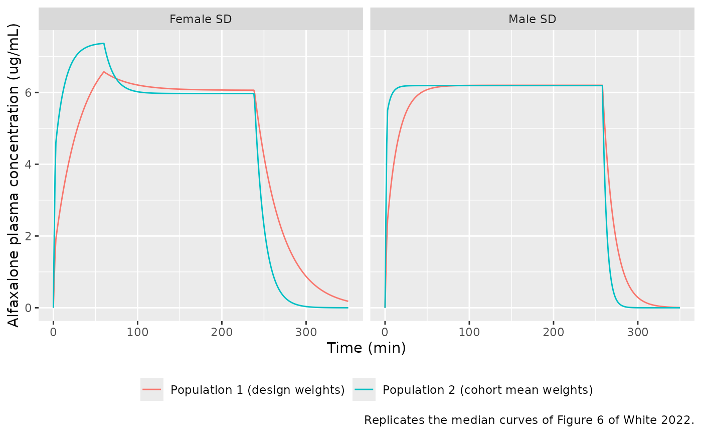
# Median curve digitised by the maintainers from Figure 6B (female SD).
fig6b <- tibble::tribble(
  ~time, ~Cc_pub,
  30,    5.18,
  40,    5.80,
  70,    6.49,
  100,   6.23,
  200,   6.08,
  250,   4.22,
  260,   3.07,
  280,   1.62,
  300,   0.85
)
fig6a <- tibble::tribble(
  ~time, ~Cc_pub,
  30,    5.70,
  40,    5.94,
  50,    6.11,
  100,   6.21,
  250,   6.21
)
cmp6 <- bind_rows(
  fig6a |> mutate(group = "Male SD"),
  fig6b |> mutate(group = "Female SD")
) |>
  left_join(f6 |> select(group, time, Cc), by = c("group", "time")) |>
  mutate(pct_diff = 100 * (Cc / Cc_pub - 1)) |>
  relocate(group)
cmp6 |>
  rename("Group" = group, "Time (min)" = time,
         "Figure 6 median (ug/mL)" = Cc_pub, "Model (ug/mL)" = Cc,
         "Difference (%)" = pct_diff) |>
knitr::kable(digits = 2, caption = "Population 1 typical profile against the digitised Figure 6 medians.")| Group | Time (min) | Figure 6 median (ug/mL) | Model (ug/mL) | Difference (%) |
|---|---|---|---|---|
| Male SD | 30 | 5.70 | 5.68 | -0.40 |
| Male SD | 40 | 5.94 | 5.95 | 0.14 |
| Male SD | 50 | 6.11 | 6.08 | -0.51 |
| Male SD | 100 | 6.21 | 6.20 | -0.21 |
| Male SD | 250 | 6.21 | 6.20 | -0.16 |
| Female SD | 30 | 5.18 | 5.12 | -1.24 |
| Female SD | 40 | 5.80 | 5.76 | -0.67 |
| Female SD | 70 | 6.49 | 6.44 | -0.81 |
| Female SD | 100 | 6.23 | 6.21 | -0.35 |
| Female SD | 200 | 6.08 | 6.07 | -0.19 |
| Female SD | 250 | 4.22 | 4.22 | 0.04 |
| Female SD | 260 | 3.07 | 3.08 | 0.37 |
| Female SD | 280 | 1.62 | 1.64 | 1.32 |
| Female SD | 300 | 0.85 | 0.87 | 2.87 |
stopifnot(
  # Digitisation reads the curve to about 0.05 ug/mL; the decay points test
  # the population 1 volume, the plateaus the clearance.
  max(abs(cmp6$pct_diff[cmp6$time <= 260])) < 3,
  max(abs(cmp6$pct_diff)) < 6
)
The population 2 model, evaluated at the actual cohort mean weights, gives the same plateaus (6.19 and 5.97 ug/mL at 200 min) as population 1 did at the design weights, but rises and decays faster because of its smaller Sprague-Dawley volume (see “Population 2 Sprague-Dawley volume” below).
Lewis-rat simulation and PKNCA
A virtual Lewis cohort (100 rats per sex, weights drawn from the Methods 2.2 means and SDs) receives the Lewis regimen: the loading infusion, 0.75 mg/kg/min to 60 min, then 0.52 mg/kg/min to 240 min, followed by a washout. Both models are simulated at typical values (the published random-effect variances are not available).
set.seed(2022)
n_per <- 100
obs_lewis <- c(0, 1, 2.5, 5, 10, 20, 30, 45, 60, 90, 120, 180, 240,
               242, 245, 250, 255, 260, 270, 280, 300, 330, 360, 420)
wt_m <- pmin(pmax(rnorm(n_per, 0.308, 0.049), 0.22), 0.45)
wt_f <- pmin(pmax(rnorm(n_per, 0.222, 0.009), 0.20), 0.25)
ev_lewis <- bind_rows(
  lapply(seq_len(n_per), function(i) {
    make_rat(i, wt_m[i], 0, 0, c(1.67, 0.75, 0.52), c(0, 2.5, 60), 240,
             obs_lewis, "Male Lewis")
  }),
  lapply(seq_len(n_per), function(i) {
    make_rat(n_per + i, wt_f[i], 1, 0, c(1.67, 0.75, 0.52), c(0, 2.5, 60), 240,
             obs_lewis, "Female Lewis")
  })
)
stopifnot(!anyDuplicated(unique(ev_lewis[, c("id", "time", "evid")])))

sim_lewis <- bind_rows(
  solve_typical(mod1, ev_lewis, keep = c("group", "WT")) |>
    mutate(model = "pop1"),
  solve_typical(mod2, ev_lewis, keep = c("group", "WT")) |>
    mutate(model = "pop2")
) |>
  mutate(treatment = paste(model, group, sep = ": "))
#> ℹ parameter labels from comments will be replaced by 'label()'
#> ℹ omega/sigma items treated as zero: 'etalcl', 'etalvc'
#> ℹ parameter labels from comments will be replaced by 'label()'
#> ℹ omega/sigma items treated as zero: 'etalcl', 'etalvc'
sim_lewis |>
  group_by(model, group, time) |>
  summarise(Q05 = quantile(Cc, 0.05), Q50 = median(Cc), Q95 = quantile(Cc, 0.95),
            .groups = "drop") |>
  ggplot(aes(time, Q50, colour = group, fill = group)) +
  geom_ribbon(aes(ymin = Q05, ymax = Q95), alpha = 0.2, colour = NA) +
  geom_line() +
  facet_wrap(~model) +
  labs(x = "Time (min)", y = "Alfaxalone plasma concentration (ug/mL)",
       colour = NULL, fill = NULL,
       caption = paste("Typical-value profiles across the weight distribution;",
                       "compare with the per-rat fits of Figure 3 of White 2022.")) +
  theme(legend.position = "bottom")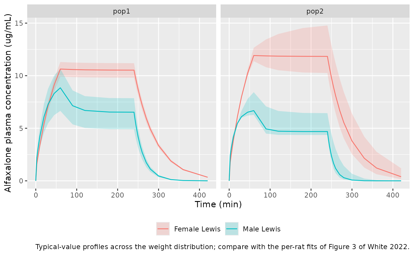
Table 2 reports the per-kg clearance and half-life of each Lewis rat
from the authors’ separate two-stage deterministic analysis (individual
fits to per-kg doses). PKNCA computes the same quantities from the
simulated profiles; dose is supplied per kg so that cl.obs
is per kg.
sim_nca <- sim_lewis |>
  filter(!is.na(Cc)) |>
  select(id, time, Cc, treatment)
sim_nca <- bind_rows(
  sim_nca,
  sim_nca |> distinct(id, treatment) |> mutate(time = 0, Cc = 0)
) |>
  distinct(id, treatment, time, .keep_all = TRUE) |>
  arrange(treatment, id, time)

dose_df <- bind_rows(
  ev_lewis |> mutate(model = "pop1"),
  ev_lewis |> mutate(model = "pop2")
) |>
  filter(evid == 1) |>
  mutate(
    treatment = paste(model, group, sep = ": "),
    amt = amt / WT,            # mg/kg
    duration = amt / (rate / WT)
  ) |>
  select(id, time, amt, duration, treatment)

conc_obj <- PKNCAconc(sim_nca, Cc ~ time | treatment + id)
dose_obj <- PKNCAdose(dose_df, amt ~ time | treatment + id, duration = "duration")
intervals <- data.frame(
  start = 0, end = Inf,
  cmax = TRUE, aucinf.obs = TRUE, cl.obs = TRUE, half.life = TRUE
)
nca_res <- pk.nca(PKNCAdata(conc_obj, dose_obj, intervals = intervals))

# cl.obs is in (mg/kg) / (ug/mL * min) = L/min/kg; report mL/min/kg.
nca_res$result <- nca_res$result |>
  mutate(PPORRES = ifelse(PPTESTCD == "cl.obs", 1000 * PPORRES, PPORRES))

published <- tibble::tribble(
  ~treatment,               ~cl.obs, ~half.life,
  "pop1: Male Lewis",       98.3,    13.5,
  "pop1: Female Lewis",     36.8,    64.7,
  "pop2: Male Lewis",       98.3,    13.5,
  "pop2: Female Lewis",     36.8,    64.7
)
cmp <- ncaComparisonTable(
  simulated = nca_res,
  reference = published,
  by = "treatment",
  params = c("cl.obs", "half.life"),
  units = c(cl.obs = "mL/min/kg", half.life = "min"),
  tolerance_pct = 20
)
knitr::kable(
  cmp,
  caption = paste("Simulated (median) vs Table 2 two-stage estimates for Lewis rats.",
                  "* differs from reference by >20%.")
)| NCA parameter | treatment | Reference | Simulated | % diff |
|---|---|---|---|---|
| t½ (min) | pop1: Male Lewis | 13.5 | 15.7 | +16.1% |
| t½ (min) | pop1: Female Lewis | 64.7 | 36.4 | -43.8%* |
| t½ (min) | pop2: Male Lewis | 13.5 | 10.1 | -25.4%* |
| t½ (min) | pop2: Female Lewis | 64.7 | 36.6 | -43.5%* |
| CL/F (mL/min/kg) | pop1: Male Lewis | 98.3 | 79.4 | -19.2% |
| CL/F (mL/min/kg) | pop1: Female Lewis | 36.8 | 49.4 | +34.4%* |
| CL/F (mL/min/kg) | pop2: Male Lewis | 98.3 | 110 | +12.3% |
| CL/F (mL/min/kg) | pop2: Female Lewis | 36.8 | 44 | +19.5% |
# PKNCA must recover the model's own clearance (a check on the dose/duration
# bookkeeping, not on the paper): AUC to infinity of a linear model.
cl_chk <- nca_res$result |>
  filter(PPTESTCD == "cl.obs") |>
  left_join(sim_lewis |> distinct(id, treatment, WT, cl), by = c("id", "treatment")) |>
  mutate(rel = PPORRES / (1000 * cl / WT) - 1)
stopifnot(quantile(abs(cl_chk$rel), 0.9, na.rm = TRUE) < 0.02)
The CL/F rows are the intravenous clearance per kg. For
male Lewis rats the population 1 clearance and half-life lie within 20%
of the Table 2 means; population 2 gives a higher clearance (+12%) and,
with its smaller Lewis volume (0.51 L), a half-life about 25% shorter
than Table 2. For female Lewis rats the half-life rows, and the
population 1 clearance, are starred: Table 2’s female half-life (64.7
min) and clearance (36.8 mL/min/kg) describe slower elimination than
either NLME model’s typical female (44-49 mL/min/kg, half-life about 36
min). Table 2 is a different analysis (per-rat fits on per-kg doses,
with a separately estimated volume for every rat; female Vdss 3.0 L/kg
against the NLME 0.57 L, i.e. about 2.6 L/kg at 222 g), and the NLME
post-hoc female Lewis clearances (40.8 mL/min/kg in Table 3, 40.4 in
Table 4) also sit below the typical values. The difference is not a
transcription error in the packaged models, whose typical values
reproduce Tables 3 and 4.
Population 2 Sprague-Dawley volume
Table 4 also lists post-hoc (empirical Bayes) mean Vd per kg. For the Lewis groups these agree with the typical Vd divided by the group mean weight; for the Sprague-Dawley groups they are 3-4 times larger than the printed typical Vd of 0.26 L would give.
vd_tab <- tibble::tribble(
  ~group,         ~WT_g, ~vd_typ, ~vd_posthoc,
  "Male Lewis",   308,   0.51,    1.58,
  "Female Lewis", 222,   0.51,    3.03,
  "Male SD",      403,   0.26,    2.18,
  "Female SD",    297,   0.26,    3.84
) |>
  mutate(vd_typ_per_kg = vd_typ / (WT_g / 1000),
         ratio = vd_posthoc / vd_typ_per_kg)
vd_tab |>
  rename("Group" = group, "Mean weight (g)" = WT_g,
         "Typical Vd, Table 4 (L)" = vd_typ,
         "Typical Vd per kg (L/kg)" = vd_typ_per_kg,
         "Post-hoc mean Vd, Table 4 (L/kg)" = vd_posthoc,
         "Post-hoc / typical" = ratio) |>
knitr::kable(digits = 2, caption = "Population 2 typical versus post-hoc volume (Sprague-Dawley weights back-solved from Table 4 CL).")| Group | Mean weight (g) | Typical Vd, Table 4 (L) | Post-hoc mean Vd, Table 4 (L/kg) | Typical Vd per kg (L/kg) | Post-hoc / typical |
|---|---|---|---|---|---|
| Male Lewis | 308 | 0.51 | 1.58 | 1.66 | 0.95 |
| Female Lewis | 222 | 0.51 | 3.03 | 2.30 | 1.32 |
| Male SD | 403 | 0.26 | 2.18 | 0.65 | 3.38 |
| Female SD | 297 | 0.26 | 3.84 | 0.88 | 4.39 |
Post-hoc means of a log-normal random effect sit close to the typical value, so a three- to four-fold excess suggests the Sprague-Dawley volume of the fit is nearer 1 L than 0.26 L, i.e. that the printed strain coefficient may have the wrong sign (0.51 * exp(+0.692) = 1.02 L). Equation 4 and the Table 4 typical value agree with each other, however, and the paper offers no independent check of the population 2 volume (Figure 6 is a population 1 simulation). The packaged model therefore follows the printed equation; users simulating Sprague-Dawley rats with population 2 should be aware that the volume, and so the loading-phase and washout kinetics, may be understated. Steady-state concentrations depend only on clearance and are unaffected.
Assumptions and deviations
-
Random effects and residual error are not reported.
The paper states that random effects were estimated on all parameters
(diagonal omega) and that a Phoenix mixed-ratio residual error was used,
but prints no variance or error magnitude in the text, tables or
supplement.
etalcl,etalvc,addSdandpropSdare held at zero; simulations are typical-value. The Figure S3/S6 box plots also show a random effect on the mixed-ratio parameter itself, which is not represented. -
Residual error form. Phoenix’s mixed ratio model,
C + CEps * (1 + C * CMixRatio), is an additive SD plus a proportional SD summed linearly, encoded asadd() + prop() + combined1(). -
LCBW base and centre. Recovered as
log10(WT / 0.317 kg)from the Figure S7 source data and confirmed against the Table 4 Lewis clearances (see Source trace). The linear form1 + 3.64 * LCBWwould give a negative clearance below about 168 g, well below the studied range (208-488 g). - Figure 6 weights. The body weights behind the Figure 6 simulation are not printed; 336 g (male) and 253 g (female) are back-solved from the plateaus and the population 1 clearances. Infusion stop times are read off the figure.
-
Strain covariate.
STRAIN_SDtakes the Lewis rat as its reference (Methods 2.8.1: Lewis = 0, SD = 1); the register entry records that the comparator strain is set per paper. - Population 2 Sprague-Dawley volume. Encoded as printed (Eq 4, exp(-0.692)); see the section above for the evidence of a possible sign error.
- Not packaged. The two-stage deterministic one-compartment fits of the individual Lewis rats (Table 2) are individual analyses rather than a population model; they are used here only as a comparator. The blood pressure observations (Figures 2, 4, 5, 7) were not modelled by the authors.
- No erratum or correction notice for this article was found (checked 2026-10-10).