Ondansetron (de Alwis 1998)
Source:vignettes/articles/deAlwis_1998_ondansetron.Rmd
deAlwis_1998_ondansetron.RmdModel and source
- Citation: de Alwis DP, Aarons L, Palmer JL. Population pharmacokinetics of ondansetron: a covariate analysis. Br J Clin Pharmacol. 1998. doi:10.1046/j.1365-2125.1998.00756.x
- Description: Two-compartment population PK model with zero-order intravenous-infusion input for ondansetron in pooled paediatric, young-adult, elderly, and aged subjects (de Alwis 1998). The paper uses an empirical additive linear-regression covariate model in the 1990s NONMEM tradition (Maitre 1991 three-step approach): clearance CL and inter-compartmental clearance CLd are sex-stratified with separate male and female intercepts and slopes; the central volume V1 has a body-weight slope only; the steady-state volume Vss has body-weight and age slopes; the peripheral volume Vp is derived as Vss - V1. Inter-individual variability is diagonal log-normal on CL, V1, Vss, and CLd. Proportional residual error is stratified across five paper-defined study sub-populations (young healthy volunteers 18-41 y, elderly healthy volunteers 61-75 y, aged healthy volunteers >= 75 y, paediatric cancer patients receiving chemotherapy, paediatric patients receiving general anaesthesia), switched at runtime via the canonical AGE / DIS_HEALTHY / DIS_CANCER_PED covariates.
- Article: https://doi.org/10.1046/j.1365-2125.1998.00756.x
Population
The model was developed from 99 subjects pooled across four phase I/II ondansetron intravenous studies (de Alwis 1998 Methods, “Data” paragraph). The training cohort spans paediatric cancer patients receiving chemotherapy, paediatric patients receiving general anaesthesia, and adult healthy volunteers stratified into young, elderly, and aged sub-cohorts. Demographics available for modelling were limited to age, weight, and gender; no race, no laboratory chemistry, no concomitant-medication, and no organ-function covariates were tested. Total 1,506 plasma concentrations were used for population analysis.
Per-sub-population breakdown (de Alwis 1998 Methods, “Data” paragraph):
- Study 1 (n = 32): adult male healthy volunteers – 16 young (18-41 y) and 16 elderly (65-75 y); single 8 mg i.v. 15-min infusion.
- Study 2 (n = 34): age-and-gender stratified healthy volunteers – young (21-38 y, 6 M + 5 F), elderly (61-74 y, 6 M + 6 F), aged (75-82 y, 5 M + 6 F); single 0.15 mg/kg i.v. 15-min infusion.
- Study 3 (n = 14): paediatric cancer patients aged 2-13 y (3 F + 11 M); single BSA-banded i.v. 15-min infusion (5 mg/m^2 if BSA <= 1.2 m^2; 8 mg flat otherwise).
- Study 4 (n = 19): paediatric patients aged 3-11 y undergoing general anaesthesia (11 F + 8 M); single 5-min i.v. infusion before anaesthetic induction (2 mg if 3-7 y; 4 mg if 8-11 y).
Combined demographics across studies 1-4: weight range 10.2-95.8 kg,
age range 2-82 y, sex split 31 female / 68 male. The same information is
available programmatically via
readModelDb("deAlwis_1998_ondansetron")$population.
Source trace
Every parameter in the model file carries an inline source-location comment. The table below collects the entries in one place.
| Equation / parameter | Value | Source location |
|---|---|---|
| Two-compartment open model with zero-order i.v.-infusion input | n/a | Results paragraph “Step 1”, “two compartment model gave a superior fit” |
| Multiplicative inter- and intra-individual error | n/a | Results paragraph “Step 1”, “inter- and intra-individual variability were best described by a multiplicative error models” |
| Five-stratum residual error by sub-population | n/a | Results paragraph “Step 1”, “separate intra-individual variance terms were used for the five groups” + Table 1 footnotes 1..5 |
| Sex coding: gender = 1 female, 0 male | n/a | Table 2 footnote “#gender 1 for females and 0 for males” |
th_cl_int_m (CL male intercept) |
5.72 L/h | Table 3, Three Step Full data, “CL male” row |
th_cl_wt_m (CL male WT slope) |
0.36 L/h/kg | Table 3, Three Step Full data, “CL male” row |
th_cl_age_m (CL male AGE slope) |
-0.17 L/h/year | Table 3, Three Step Full data, “CL male” row |
th_cl_int_f (CL female intercept) |
7.78 L/h | Table 3, Three Step Full data, “CL female” row |
th_cl_wt_f (CL female WT slope) |
0.20 L/h/kg | Table 3, Three Step Full data, “CL female” row |
th_cl_age_f (CL female AGE slope) |
-0.04 L/h/year | Table 3, Three Step Full data, “CL female” row |
th_v1_int (V1 intercept) |
8.08 L | Table 3, Three Step Full data, “V1” row |
th_v1_wt (V1 WT slope) |
0.31 L/kg | Table 3, Three Step Full data, “V1” row |
th_vss_int (Vss intercept) |
4.79 L | Table 3, Three Step Full data, “Vss” row |
th_vss_wt (Vss WT slope) |
1.88 L/kg | Table 3, Three Step Full data, “Vss” row |
th_vss_age (Vss AGE slope) |
0.133 L/year | Table 3, Three Step Full data, “Vss” row |
th_cld_int_m (CLd male intercept) |
-22.3 L/h | Table 3, Three Step Full data, “CLd male” row |
th_cld_wt_m (CLd male WT slope) |
3.89 L/h/kg | Table 3, Three Step Full data, “CLd male” row |
th_cld_int_f (CLd female intercept) |
-76.9 L/h | Table 3, Three Step Full data, “CLd female” row |
th_cld_wt_f (CLd female WT slope) |
7.49 L/h/kg | Table 3, Three Step Full data, “CLd female” row |
| Vp = max(Vss - V1, 0.01 L) | derived | Standard 2-cmt identity |
| IIV CL (CV%) | 29.6% | Table 1, Final covariate model, All data, CL row |
| IIV V1 (CV%) | 71.1% | Table 1, Final covariate model, All data, V1 row |
| IIV Vss (CV%) | 36.7% | Table 1, Final covariate model, All data, Vss row |
| IIV CLd (CV%) | 37.0% | Table 1, Final covariate model, All data, CLd row |
propSd_young_vol (group *1) |
12.5% | Table 1, Final covariate model, All data, group *1 |
propSd_elderly_vol (group *2) |
13.3% | Table 1, Final covariate model, All data, group *2 |
propSd_aged_vol (group *3) |
16.9% | Table 1, Final covariate model, All data, group *3 |
propSd_paed_chemo (group *4) |
17.8% | Table 1, Final covariate model, All data, group *4 |
propSd_paed_anaes (group *5) |
14.5% | Table 1, Final covariate model, All data, group *5 |
Virtual cohort
Original observed ondansetron concentrations from the four phase I/II studies are not openly available. The virtual cohort below mirrors the per-study demographics from de Alwis 1998 Methods “Data” paragraph as closely as the reported summary statistics allow (uniform sampling within the reported age and weight ranges; sex assigned to match the per-study female fractions recorded in the text).
set.seed(19980401)

make_cohort <- function(n,
                        age_lo, age_hi,
                        wt_lo, wt_hi,
                        sex_female_pct,
                        dis_healthy, dis_cancer_ped,
                        dose_mg, dose_dur_h,
                        label, id_offset) {
  age <- runif(n, age_lo, age_hi)
  wt  <- runif(n, wt_lo, wt_hi)
  sexf <- as.integer(runif(n) < sex_female_pct / 100)
  dose_subject <- if (length(dose_mg) == 1L) rep(dose_mg, n) else dose_mg
  dose_dur     <- if (length(dose_dur_h) == 1L) rep(dose_dur_h, n) else dose_dur_h
  ids <- id_offset + seq_len(n)

  # Build per-subject dose + observation rows. 15-min infusion (5-min for the
  # paediatric-anaesthesia cohort) into the central compartment; observation
  # grid spans 24 h to capture distribution and elimination.
  obs_grid <- c(0, 0.083, 0.167, 0.25, 0.333, 0.417, 0.5, 0.75,
                1, 1.5, 2, 3, 4, 5, 6, 8, 10, 12, 18, 24)

  dose_rows <- tibble(
    id   = ids, time = 0, amt = dose_subject, evid = 1L,
    cmt  = "central", dur = dose_dur,
    WT = wt, AGE = age, SEXF = sexf,
    DIS_HEALTHY = dis_healthy, DIS_CANCER_PED = dis_cancer_ped,
    cohort = label
  )

  obs_rows <- tidyr::crossing(id = ids, time = obs_grid) |>
    mutate(amt = 0, evid = 0L, cmt = "central", dur = 0) |>
    left_join(dose_rows |> select(id, WT, AGE, SEXF,
                                  DIS_HEALTHY, DIS_CANCER_PED, cohort),
              by = "id")

  bind_rows(dose_rows, obs_rows) |> arrange(id, time, desc(evid))
}

# Young healthy volunteers (study 1 young + study 2 young).
# Studies pool to AGE 18-41 y; mixed sex (study 1 was all male, study 2 had
# 5/11 female; pooled female fraction ~ 18%).
young_vol <- make_cohort(
  n = 100,
  age_lo = 18, age_hi = 41,
  wt_lo  = 55, wt_hi = 85,
  sex_female_pct = 18,
  dis_healthy = 1L, dis_cancer_ped = 0L,
  dose_mg = 8, dose_dur_h = 0.25,
  label = "Young volunteers (study 1+2)",
  id_offset = 0L
)

# Elderly healthy volunteers (study 1 elderly + study 2 elderly).
# Studies pool to AGE 61-75 y; mixed sex.
elderly_vol <- make_cohort(
  n = 100,
  age_lo = 61, age_hi = 75,
  wt_lo  = 55, wt_hi = 95,
  sex_female_pct = 27,
  dis_healthy = 1L, dis_cancer_ped = 0L,
  dose_mg = 8, dose_dur_h = 0.25,
  label = "Elderly volunteers (study 1+2)",
  id_offset = 200L
)

# Aged healthy volunteers (study 2 aged). AGE 75-82 y; 5 M / 6 F.
aged_vol <- make_cohort(
  n = 80,
  age_lo = 75, age_hi = 82,
  wt_lo  = 50, wt_hi = 90,
  sex_female_pct = 55,
  dis_healthy = 1L, dis_cancer_ped = 0L,
  dose_mg = 8, dose_dur_h = 0.25,
  label = "Aged volunteers (study 2)",
  id_offset = 400L
)

# Paediatric chemotherapy (study 3). AGE 2-13 y; weight from a piecewise
# weight-for-age curve (Chumlea / WHO reference smoothed) so the cohort
# spans the published 10.2-95.8 kg range realistically.
paed_age_to_wt <- function(age_y) pmax(8, 8 + 2.4 * age_y + rnorm(length(age_y), 0, 3))

paed_chemo_age <- runif(80, 2, 13)
paed_chemo_wt  <- paed_age_to_wt(paed_chemo_age)
# BSA-banded dose: 5 mg/m^2 if BSA <= 1.2 m^2, 8 mg otherwise. Approximate
# BSA via DuBois: 0.007184 * WT^0.425 * HT^0.725; pediatric height from
# height-for-age (rough): HT_cm ~ 75 + 6 * AGE_y for AGE 2-13.
paed_chemo_ht  <- 75 + 6 * paed_chemo_age
paed_chemo_bsa <- 0.007184 * paed_chemo_wt^0.425 * paed_chemo_ht^0.725
paed_chemo_dose <- ifelse(paed_chemo_bsa <= 1.2, 5 * paed_chemo_bsa, 8)

paed_chemo <- (function() {
  n <- 80; id_offset <- 600L
  ids <- id_offset + seq_len(n)
  sexf <- as.integer(runif(n) < 0.21)  # 3 / 14 female

  obs_grid <- c(0, 0.083, 0.167, 0.25, 0.5, 1, 2, 3, 4, 5, 6, 8, 10, 12)

  dose_rows <- tibble(
    id   = ids, time = 0, amt = paed_chemo_dose, evid = 1L,
    cmt  = "central", dur = 0.25,
    WT = paed_chemo_wt, AGE = paed_chemo_age, SEXF = sexf,
    DIS_HEALTHY = 0L, DIS_CANCER_PED = 1L,
    cohort = "Paediatric chemo (study 3)"
  )
  obs_rows <- tidyr::crossing(id = ids, time = obs_grid) |>
    mutate(amt = 0, evid = 0L, cmt = "central", dur = 0) |>
    left_join(dose_rows |> select(id, WT, AGE, SEXF,
                                  DIS_HEALTHY, DIS_CANCER_PED, cohort),
              by = "id")
  bind_rows(dose_rows, obs_rows) |> arrange(id, time, desc(evid))
})()

# Paediatric general anaesthesia (study 4). AGE 3-11 y; 11 F / 8 M (58%).
# Dose 2 mg if AGE 3-7, 4 mg if AGE 8-11. 5-min infusion.
paed_anaes_age <- runif(80, 3, 11)
paed_anaes_wt  <- paed_age_to_wt(paed_anaes_age)
paed_anaes_dose <- ifelse(paed_anaes_age < 8, 2, 4)

paed_anaes <- (function() {
  n <- 80; id_offset <- 800L
  ids <- id_offset + seq_len(n)
  sexf <- as.integer(runif(n) < 0.58)

  obs_grid <- c(0, 0.083, 0.167, 0.25, 0.5, 1, 2, 3, 4, 5, 6, 8, 10, 12)

  dose_rows <- tibble(
    id   = ids, time = 0, amt = paed_anaes_dose, evid = 1L,
    cmt  = "central", dur = 0.083,
    WT = paed_anaes_wt, AGE = paed_anaes_age, SEXF = sexf,
    DIS_HEALTHY = 0L, DIS_CANCER_PED = 0L,
    cohort = "Paediatric anaesthesia (study 4)"
  )
  obs_rows <- tidyr::crossing(id = ids, time = obs_grid) |>
    mutate(amt = 0, evid = 0L, cmt = "central", dur = 0) |>
    left_join(dose_rows |> select(id, WT, AGE, SEXF,
                                  DIS_HEALTHY, DIS_CANCER_PED, cohort),
              by = "id")
  bind_rows(dose_rows, obs_rows) |> arrange(id, time, desc(evid))
})()

events <- bind_rows(young_vol, elderly_vol, aged_vol, paed_chemo, paed_anaes)

# Disjoint-ID guard (per replicate-author-structure conventions).
stopifnot(!anyDuplicated(unique(events[, c("id", "time", "evid")])))
Simulation
mod <- readModelDb("deAlwis_1998_ondansetron")
sim <- rxode2::rxSolve(
  mod, events = events,
  keep = c("cohort", "WT", "AGE", "SEXF")
) |>
  as.data.frame() |>
  filter(time > 0)  # drop the time = 0 record for clarity in plots
#> ℹ parameter labels from comments will be replaced by 'label()'
For typical-value replications (no IIV, no residual), use:
mod_typical <- mod |> rxode2::zeroRe()
#> ℹ parameter labels from comments will be replaced by 'label()'
#> Warning: No sigma parameters in the model
sim_typical <- rxode2::rxSolve(
  mod_typical, events = events,
  keep = c("cohort", "WT", "AGE", "SEXF")
) |>
  as.data.frame() |>
  filter(time > 0)
#> ℹ omega/sigma items treated as zero: 'etalcl', 'etalvc', 'etalvss', 'etalq'
#> Warning: multi-subject simulation without without 'omega'
Replicate Figure 2 – covariate effects on CL and Vss
de Alwis 1998 Figure 2 plots empirical Bayes estimates of CL and Vss against covariates (weight, age, gender). We replicate the structural covariate model underlying those scatterplots by evaluating the typical-value CL and Vss across a grid of WT and AGE for each sex.
grid <- tidyr::crossing(
  WT   = seq(10, 95, by = 5),
  AGE  = c(5, 25, 45, 70, 80),
  SEXF = 0:1
) |>
  mutate(
    cl_male    = 5.72 + 0.36 * WT - 0.17 * AGE,
    cl_female  = 7.78 + 0.20 * WT - 0.04 * AGE,
    CL_typ     = (1 - SEXF) * cl_male + SEXF * cl_female,
    Vss_typ    = 4.79 + 1.88 * WT + 0.133 * AGE,
    sex_label  = ifelse(SEXF == 1L, "female", "male")
  )

p_cl <- ggplot(grid, aes(WT, CL_typ, colour = factor(AGE), linetype = sex_label)) +
  geom_line() +
  labs(x = "Body weight (kg)", y = "Typical CL (L/h)",
       colour = "AGE (y)", linetype = "Sex",
       title = "Figure 2a/b/e -- Typical CL vs WT, stratified by AGE and sex",
       caption = "Replicates structure of Figure 2a/b/e of de Alwis 1998 using the published linear-regression coefficients.")

p_vss <- ggplot(grid |> filter(SEXF == 0L),
                aes(WT, Vss_typ, colour = factor(AGE))) +
  geom_line() +
  labs(x = "Body weight (kg)", y = "Typical Vss (L)",
       colour = "AGE (y)",
       title = "Figure 2c/d -- Typical Vss vs WT, stratified by AGE",
       caption = "Replicates structure of Figure 2c/d of de Alwis 1998 (sex-independent).")

print(p_cl)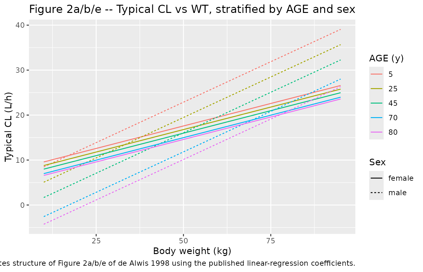
print(p_vss)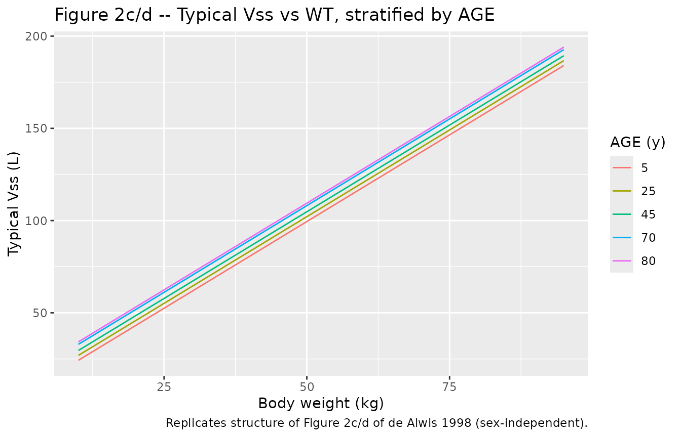
Replicate Figure 3 – basic vs covariate-model CL comparison
de Alwis 1998 Figure 3 compares CL between the basic two-compartment model and the three-step / stepwise-A covariate model for three reference subjects: a 57 kg / 37 y young adult, a 26 kg / 10 y child, and an 80 kg / 75 y elderly subject, each in both sexes. The basic-model typical CL is 20.9 L/h (Table 1, Final covariate model row); the covariate-model CL is the sex-specific linear regression evaluated at each (WT, AGE) pair.
fig3 <- tibble::tribble(
  ~subject,           ~WT, ~AGE,
  "Child (10 y, 26 kg)",  26, 10,
  "Young (37 y, 57 kg)",  57, 37,
  "Elderly (75 y, 80 kg)", 80, 75
) |>
  tidyr::crossing(SEXF = 0:1) |>
  mutate(
    cl_male    = 5.72 + 0.36 * WT - 0.17 * AGE,
    cl_female  = 7.78 + 0.20 * WT - 0.04 * AGE,
    `Covariate CL` = (1 - SEXF) * cl_male + SEXF * cl_female,
    `Basic CL`     = 20.9,
    Sex            = ifelse(SEXF == 1L, "female", "male")
  ) |>
  select(subject, Sex, `Basic CL`, `Covariate CL`)

knitr::kable(
  fig3,
  digits  = 2,
  caption = paste(
    "Figure 3 reconstruction: basic two-compartment CL vs the final",
    "covariate-model CL (three-step / full data, Table 3) for the three",
    "reference subjects of de Alwis 1998 Figure 3."
  )
)| subject | Sex | Basic CL | Covariate CL |
|---|---|---|---|
| Child (10 y, 26 kg) | male | 20.9 | 13.38 |
| Child (10 y, 26 kg) | female | 20.9 | 12.58 |
| Elderly (75 y, 80 kg) | male | 20.9 | 21.77 |
| Elderly (75 y, 80 kg) | female | 20.9 | 20.78 |
| Young (37 y, 57 kg) | male | 20.9 | 19.95 |
| Young (37 y, 57 kg) | female | 20.9 | 17.70 |
PKNCA validation
Cmax, Tmax, AUC0-inf, and half-life by simulated cohort, computed with PKNCA. The treatment grouping carries the per-cohort label through the formula so results are reported per sub-population.
sim_nca <- sim |>
  filter(!is.na(Cc), Cc > 0) |>
  select(id, time, Cc, cohort)

conc_obj <- PKNCA::PKNCAconc(
  sim_nca, Cc ~ time | cohort + id,
  concu = "ng/mL", timeu = "h"
)

dose_df <- events |>
  filter(evid == 1L) |>
  select(id, time, amt, cohort)

dose_obj <- PKNCA::PKNCAdose(
  dose_df, amt ~ time | cohort + id,
  doseu = "mg"
)

intervals <- data.frame(
  start       = 0,
  end         = Inf,
  cmax        = TRUE,
  tmax        = TRUE,
  aucinf.obs  = TRUE,
  half.life   = TRUE
)

nca_res <- suppressWarnings(
  PKNCA::pk.nca(PKNCA::PKNCAdata(conc_obj, dose_obj, intervals = intervals))
)

nca_summary <- as.data.frame(nca_res$result) |>
  group_by(cohort, PPTESTCD) |>
  summarise(
    median = median(PPORRES, na.rm = TRUE),
    q05    = quantile(PPORRES, 0.05, na.rm = TRUE),
    q95    = quantile(PPORRES, 0.95, na.rm = TRUE),
    .groups = "drop"
  ) |>
  arrange(cohort, PPTESTCD)

knitr::kable(
  nca_summary,
  digits  = 3,
  caption = "Simulated NCA parameters (median and 5/95 percentiles) by sub-population."
)| cohort | PPTESTCD | median | q05 | q95 |
|---|---|---|---|---|
| Aged volunteers (study 2) | adj.r.squared | 1.000 | 1.000 | 1.000 |
| Aged volunteers (study 2) | aucinf.obs | NA | NA | NA |
| Aged volunteers (study 2) | clast.obs | 3.254 | 0.231 | 9.937 |
| Aged volunteers (study 2) | clast.pred | 3.250 | 0.231 | 9.935 |
| Aged volunteers (study 2) | cmax | 99.520 | 61.655 | 173.653 |
| Aged volunteers (study 2) | half.life | 6.346 | 2.894 | 12.975 |
| Aged volunteers (study 2) | lambda.z | 0.109 | 0.053 | 0.240 |
| Aged volunteers (study 2) | lambda.z.n.points | 14.000 | 12.000 | 16.000 |
| Aged volunteers (study 2) | lambda.z.time.first | 0.500 | 0.333 | 1.000 |
| Aged volunteers (study 2) | lambda.z.time.last | 24.000 | 24.000 | 24.000 |
| Aged volunteers (study 2) | r.squared | 1.000 | 1.000 | 1.000 |
| Aged volunteers (study 2) | span.ratio | 3.682 | 1.810 | 8.175 |
| Aged volunteers (study 2) | tlast | 24.000 | 24.000 | 24.000 |
| Aged volunteers (study 2) | tmax | 0.250 | 0.250 | 0.250 |
| Elderly volunteers (study 1+2) | adj.r.squared | 1.000 | 1.000 | 1.000 |
| Elderly volunteers (study 1+2) | aucinf.obs | NA | NA | NA |
| Elderly volunteers (study 1+2) | clast.obs | 2.496 | 0.138 | 9.089 |
| Elderly volunteers (study 1+2) | clast.pred | 2.495 | 0.137 | 9.087 |
| Elderly volunteers (study 1+2) | cmax | 105.819 | 59.244 | 186.473 |
| Elderly volunteers (study 1+2) | half.life | 5.310 | 2.801 | 11.635 |
| Elderly volunteers (study 1+2) | lambda.z | 0.131 | 0.060 | 0.248 |
| Elderly volunteers (study 1+2) | lambda.z.n.points | 14.000 | 12.000 | 16.000 |
| Elderly volunteers (study 1+2) | lambda.z.time.first | 0.500 | 0.333 | 1.000 |
| Elderly volunteers (study 1+2) | lambda.z.time.last | 24.000 | 24.000 | 24.000 |
| Elderly volunteers (study 1+2) | r.squared | 1.000 | 1.000 | 1.000 |
| Elderly volunteers (study 1+2) | span.ratio | 4.433 | 2.001 | 8.421 |
| Elderly volunteers (study 1+2) | tlast | 24.000 | 24.000 | 24.000 |
| Elderly volunteers (study 1+2) | tmax | 0.250 | 0.250 | 0.250 |
| Paediatric anaesthesia (study 4) | adj.r.squared | 1.000 | 1.000 | 1.000 |
| Paediatric anaesthesia (study 4) | aucinf.obs | NA | NA | NA |
| Paediatric anaesthesia (study 4) | clast.obs | 3.148 | 0.357 | 10.557 |
| Paediatric anaesthesia (study 4) | clast.pred | 3.144 | 0.357 | 10.557 |
| Paediatric anaesthesia (study 4) | cmax | 138.720 | 47.355 | 318.116 |
| Paediatric anaesthesia (study 4) | half.life | 3.081 | 1.544 | 7.175 |
| Paediatric anaesthesia (study 4) | lambda.z | 0.225 | 0.097 | 0.449 |
| Paediatric anaesthesia (study 4) | lambda.z.n.points | 10.000 | 8.000 | 12.000 |
| Paediatric anaesthesia (study 4) | lambda.z.time.first | 0.500 | 0.167 | 2.000 |
| Paediatric anaesthesia (study 4) | lambda.z.time.last | 12.000 | 12.000 | 12.000 |
| Paediatric anaesthesia (study 4) | r.squared | 1.000 | 1.000 | 1.000 |
| Paediatric anaesthesia (study 4) | span.ratio | 3.605 | 1.486 | 7.652 |
| Paediatric anaesthesia (study 4) | tlast | 12.000 | 12.000 | 12.000 |
| Paediatric anaesthesia (study 4) | tmax | 0.083 | 0.083 | 0.083 |
| Paediatric chemo (study 3) | adj.r.squared | 1.000 | 1.000 | 1.000 |
| Paediatric chemo (study 3) | aucinf.obs | NA | NA | NA |
| Paediatric chemo (study 3) | clast.obs | 3.776 | 0.336 | 13.318 |
| Paediatric chemo (study 3) | clast.pred | 3.770 | 0.336 | 13.313 |
| Paediatric chemo (study 3) | cmax | 164.983 | 89.541 | 261.598 |
| Paediatric chemo (study 3) | half.life | 2.831 | 1.447 | 5.706 |
| Paediatric chemo (study 3) | lambda.z | 0.245 | 0.121 | 0.479 |
| Paediatric chemo (study 3) | lambda.z.n.points | 9.000 | 8.000 | 10.000 |
| Paediatric chemo (study 3) | lambda.z.time.first | 1.000 | 0.500 | 2.000 |
| Paediatric chemo (study 3) | lambda.z.time.last | 12.000 | 12.000 | 12.000 |
| Paediatric chemo (study 3) | r.squared | 1.000 | 1.000 | 1.000 |
| Paediatric chemo (study 3) | span.ratio | 3.839 | 1.859 | 7.707 |
| Paediatric chemo (study 3) | tlast | 12.000 | 12.000 | 12.000 |
| Paediatric chemo (study 3) | tmax | 0.250 | 0.250 | 0.250 |
| Young volunteers (study 1+2) | adj.r.squared | 1.000 | 1.000 | 1.000 |
| Young volunteers (study 1+2) | aucinf.obs | NA | NA | NA |
| Young volunteers (study 1+2) | clast.obs | 0.907 | 0.042 | 5.855 |
| Young volunteers (study 1+2) | clast.pred | 0.906 | 0.042 | 5.843 |
| Young volunteers (study 1+2) | cmax | 109.568 | 66.782 | 164.319 |
| Young volunteers (study 1+2) | half.life | 4.206 | 2.196 | 8.684 |
| Young volunteers (study 1+2) | lambda.z | 0.165 | 0.080 | 0.316 |
| Young volunteers (study 1+2) | lambda.z.n.points | 14.000 | 11.950 | 16.000 |
| Young volunteers (study 1+2) | lambda.z.time.first | 0.500 | 0.333 | 1.025 |
| Young volunteers (study 1+2) | lambda.z.time.last | 24.000 | 24.000 | 24.000 |
| Young volunteers (study 1+2) | r.squared | 1.000 | 1.000 | 1.000 |
| Young volunteers (study 1+2) | span.ratio | 5.558 | 2.707 | 10.750 |
| Young volunteers (study 1+2) | tlast | 24.000 | 24.000 | 24.000 |
| Young volunteers (study 1+2) | tmax | 0.250 | 0.250 | 0.250 |
Comparison against the basic-model typical values
de Alwis 1998 reports basic-model typical PK parameters in Table 1 (Final covariate model column, All data row): CL = 20.9 L/h, V1 = 24.9 L, Vss = 146.9 L, CLd = 252.0 L/h. The covariate-model AUC0-inf for a typical 70 kg subject given an 8 mg single i.v. dose should approximate 8 mg / 20.9 L/h ~ 383 ngh/mL (basic) or 8 mg / 24.6 L/h ~ 325 ngh/mL (covariate, 37 y male). The simulated Young-Volunteer cohort median AUC above is the relevant comparison row.
basic_pred <- tibble::tibble(
  cohort       = "Young volunteers (study 1+2)",
  basic_AUC    = 8 * 1000 / 20.9,
  covar_AUC_male_37y = 8 * 1000 / 24.63
)
knitr::kable(
  basic_pred,
  digits  = 1,
  caption = "Reference AUC0-inf (ng*h/mL) implied by the basic two-compartment CL and by the covariate-model typical CL for a 37 y / 70 kg male."
)| cohort | basic_AUC | covar_AUC_male_37y |
|---|---|---|
| Young volunteers (study 1+2) | 382.8 | 324.8 |
Replicate Figure 1 – visual residual check
de Alwis 1998 Figure 1 shows weighted residuals from the NONMEM fit for the five sub-populations against population predictions, with the lack of fit in the paediatric groups visible in panel (a) (basic model) and reduced in panel (b) (final covariate model). The simulated data here come from the final covariate model, so the analogous plot below uses simulated concentrations and the typical-value population prediction as the abscissa to show the residual distribution under the final structure.
sim_pred <- left_join(
  sim |> select(id, time, cohort, Cc),
  sim_typical |> select(id, time, Cc_typ = Cc),
  by = c("id", "time")
) |>
  mutate(
    wres = (Cc - Cc_typ) / pmax(Cc_typ, 0.01)
  ) |>
  filter(!is.na(Cc_typ), Cc_typ > 1)

ggplot(sim_pred, aes(Cc_typ, wres, colour = cohort)) +
  geom_hline(yintercept = 0, linetype = 2, colour = "grey50") +
  geom_point(alpha = 0.2, size = 0.5) +
  scale_x_log10() +
  labs(x = "Typical-value (population) Cc (ng/mL)", y = "Standardised residual",
       title = "Figure 1b analogue -- weighted residuals from the final covariate model",
       caption = "Replicates structure of Figure 1b of de Alwis 1998 using simulated data from the packaged model.") +
  theme(legend.position = "bottom")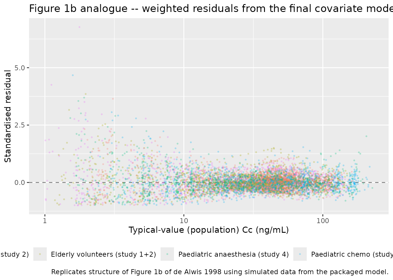
Assumptions and deviations
Empirical additive linear-regression covariate model. The published paper uses a 1990s-NONMEM-tradition additive linear-regression covariate model (Maitre 1991 three-step approach) for all four structural PK parameters rather than the log-linear / allometric / power forms standard in modern popPK. The structural-parameter coefficients in
ini()carry paper-specificth_<param>_<term>names (intercepts and per-covariate slopes for males and females) that do not match the canonicallcl/lvc/lqpatterns or the canonicale_<cov>_<param>covariate- effect prefix; thepaper_specific_etasmetadata field declaresetalcl/etalvc/etalvss/etalqso the convention checker accepts the eta names that pair with the derived typical-value parameters computed insidemodel()rather than withini()lXparameters.Linear regression yields negative typical values for extreme covariate combinations. A 10 kg / 82 y subject yields a negative
cl_typ_male(5.72 + 3.60 - 13.94 = -4.62 L/h), and a 10 kg female yields a slightly negativecld_typ_female(-76.9 + 74.9 = -2.0 L/h). The published training cohort never combines such extreme weights with extreme ages (paediatric subjects in studies 3 and 4 are 2-13 y; aged volunteers in study 2 are 75-82 y with weights 50-90 kg), so the linear-regression domain of validity is the joint weight x age range of the four training studies, not the marginal ranges. Simulating outside that joint domain may produce non-physiological negative clearances. Thevpperipheral volume carries amax(vss - vc, 0.01 L)floor insidemodel()to keep the ODE micro-constants finite under IIV draws whereexp(etalvc)shifts Vc above the realised Vss.Sex stratification implemented as separate male and female equations. de Alwis 1998 Table 3 reports the final covariate model as two parallel CL equations (CL male = 5.72 + 0.36WT - 0.17AGE; CL female = 7.78 + 0.20WT - 0.04AGE) and two parallel CLd equations (CLd male = -22.3 + 3.89WT; CLd female = -76.9 + 7.49WT). The model file evaluates both equations in
model()and dispatches by SEXF (1 = female, 0 = male, matching the paper’s coding). V1 and Vss are not sex-stratified.Five-stratum proportional residual error switched via existing canonical covariates. Rather than introducing a new categorical
POP_GROUPcovariate, the model uses combinations of the existing canonical AGE, DIS_HEALTHY (1 = healthy volunteer, 0 = paediatric patient), and DIS_CANCER_PED (1 = paediatric chemotherapy, 0 = other) covariates to dispatch the per-subject proportional-residual-error magnitude across the five paper-defined sub-populations. AGE thresholds 45 y and 75 y separate the paper’s three volunteer age bands (young < 45 y, elderly 45-75 y, aged >= 75 y). At inference time exactly one of the five indicator products is 1 for any given subject.Volunteer-vs-patient cohort assignment for non-training-cohort subjects. Within the training cohort all DIS_HEALTHY = 0 subjects are paediatric (studies 3 and 4); the residual-error switch routes them into one of the two paediatric strata via DIS_CANCER_PED. Adult patients (e.g., the test-set adult cancer cohort in study 6) were not in the training set, and the model does not have a residual-error stratum for them. Users simulating adult patients should treat the choice of propSd stratum as a model assumption rather than an estimated quantity.
Bioanalysis heterogeneity drives the residual-error stratification. de Alwis 1998 Methods note that “plasma samples for the different studies were analysed by different centres”, which is one of the sources of the residual-error heterogeneity across the five sub- populations. The single-laboratory bioanalysis assumption inherent in pooled population PK is therefore relaxed at the residual-error level in the published model.
Virtual cohort uses synthetic demographics. The virtual cohort in this vignette samples ages and weights uniformly within the per-study ranges reported in de Alwis 1998 Methods and assigns sex from the per-study female fractions. The original individual-level demographics are not openly available; the synthetic distributions are only meant to span the training-cohort domain so per-stratum NCA comparisons can be drawn against the basic-model expectations summarised in Table 1.
Test-set predictions (studies 5-7) are not replicated here. de Alwis 1998 Results validate the final covariate model against an independent 54-subject test set (studies 5-7) via standardised prediction errors at three time points (0.25 h, 1 h, 8 h post dose). The test-set validation is documented in Figures 5 and 6 of the source. This vignette focuses on the training-set sub-population behaviour and the typical-value covariate-model replication; test-set SPE reconstruction would require the published per-subject test-set demographics, which are not openly available.
Bioavailability not modelled. All doses in the four training studies were intravenous; bioavailability is implicit in the parameter scale (F = 1) and no depot compartment is needed.