Dutogliptin (Marier 2014) • nlmixr2lib

Model and source

mod <- readModelDb("Marier_2014_dutogliptin")
ui  <- rxode2::rxode(mod)
#> ℹ parameter labels from comments will be replaced by 'label()'

Citation: Marier JF, Mouksassi MS, Gosselin NH, Li J. Population Pharmacokinetic Analysis of Dutogliptin, a Selective Dipeptidyl Peptidase-4 Inhibitor. Clin Pharmacol Drug Dev. 2014;3(4):297-304. doi:10.1002/cpdd.87
Description: Two-compartment population PK model with a lag time and formulation-specific first-order absorption for dutogliptin, a selective dipeptidyl peptidase-4 inhibitor, in healthy subjects and patients with type 2 diabetes mellitus (Marier 2014)
Article: https://doi.org/10.1002/cpdd.87
Supplement (Tables S1-S3, Figures S1-S2): https://doi.org/10.1002/cpdd.87, “Supporting Information”

Dutogliptin (PHX1149) is a selective, orally administered dipeptidyl peptidase-4 (DPP-4) inhibitor that was in late-stage development for type 2 diabetes mellitus (T2DM). It is hydrophilic, highly water soluble, minimally protein bound and minimally metabolised, and is excreted as parent compound in urine; Marier 2014 notes that its apparent clearance is close to the glomerular filtration rate, which is why creatinine clearance is the dominant covariate on CL/F.

Population

The analysis pooled 561 subjects from nine studies (Marier 2014 Table 1, Supplemental Tables S1 and S2): 144 healthy subjects and patients contributing 2,933 measurable concentrations across seven Phase I studies (PROT101, PROT102, PROT103, PROT104, PROT107, PROT109, PROT110), and 417 patients with T2DM contributing 2,153 measurable concentrations across two Phase II studies (PROT201, PROT202). Doses ranged from 50 to 500 mg, given as an aqueous solution, a free-base hard-shell capsule, an enteric-coated capsule, or a tartrate-salt tablet, under fasting and several fed conditions. PROT107 enrolled subjects with normal through severe renal impairment; PROT109 assessed co-administration with metformin in patients with T2DM.

Mean age was 52.7 years (range 18 to 77; 52 subjects were older than 65) and mean weight 85.5 kg (median 82.5, range 44.6 to 158.6). Mean Cockcroft-Gault creatinine clearance was 117.5 mL/min (median 111.0, range 25.4 to 329.3). The cohort was 49.73% female and 63.99% Caucasian, 19.61% Other, 12.66% Asian and 3.74% Black. The assay LOQ was 1 ng/mL and the model was fitted in NONMEM VI.

str(ui$population)
#> List of 15
#>  $ species       : chr "human"
#>  $ n_subjects    : num 561
#>  $ n_studies     : num 9
#>  $ age_range     : chr "18-77 years"
#>  $ age_median    : chr "54 years"
#>  $ weight_range  : chr "44.6-158.6 kg"
#>  $ weight_median : chr "82.5 kg"
#>  $ sex_female_pct: num 49.7
#>  $ race_ethnicity: Named num [1:4] 63.99 12.66 3.74 19.61
#>   ..- attr(*, "names")= chr [1:4] "Caucasian" "Asian" "Black" "Other"
#>  $ disease_state : chr "Healthy subjects and patients with type 2 diabetes mellitus; includes a dedicated renal-impairment study (PROT1"| __truncated__
#>  $ dose_range    : chr "50-500 mg orally, single and once-daily repeated doses"
#>  $ renal_function: chr "Creatinine clearance (Cockcroft-Gault) mean 117.5 mL/min, median 111.0, range 25.4-329.3 mL/min; truncated at 1"| __truncated__
#>  $ co_medication : chr "Phase II subjects were on stable metformin, or metformin plus a thiazolidinedione."
#>  $ formulations  : chr "Aqueous solution, free-base hard-shell capsule, enteric-coated capsule, and tartrate-salt tablet."
#>  $ notes         : chr "Demographics from Marier 2014 Table 1 (pooled Phase I and Phase II). 144 subjects contributed 2,933 measurable "| __truncated__

Source trace

Every ini() entry carries an in-file comment naming its source location in inst/modeldb/specificDrugs/Marier_2014_dutogliptin.R. They are collected here for review. Two rows are not paper-printed values and are flagged as such; see “Assumptions and deviations” below.

Equation / parameter	Value	Source location
Structure: two-compartment, first-order absorption, lag time	n/a	Abstract; Results, “Population PK Analysis of Dutogliptin”
`lka_cap` (capsule and aqueous solution)	1.55 1/h	Table 2, “1.55 for capsules”; Results p.302 for the solution (“comparable to that of the capsules”)
`lka_tab` (tartrate-salt tablet)	0.558 1/h	Table 2, “0.558 for tablets”
`lka_ec` (enteric-coated capsule)	0.0204 1/h	Results p.302, “the enteric-coated capsules displayed much slower absorption (0.0204 hour-1)”
`tlag` (absorption lag time)	`fixed(0)`	NOT REPORTED. Named as a model component in the Abstract, Methods p.299 and Results p.302, but no value is printed anywhere in the paper or supplement
`lcl` (CL/F at CrCL 115.7 mL/min)	176 L/h	Table 2, `CL/F = 176 * (CrCL / 115.7)^0.848`
`e_crcl_cl`	0.848	Table 2 (same equation)
`lvc` (Vc/F at 82.5 kg)	1250 L	BACK-SOLVED from Table 2 `Vss/F = 2041 L` plus the three printed terminal half-lives (Results p.302-303)
`lvp` (Vp/F at 82.5 kg)	791 L	BACK-SOLVED; `2041 - 1250` preserves the printed Vss/F exactly
`lq` (Q/F)	78.6 L/h	BACK-SOLVED from the same three (CL/F, t1/2) pairs
`e_wt_vc_vp`	1.0	Table 2, `Vss/F = 2041 * (Body Weight / 82.5)^1.0`
`e_race_black_vc_vp`	0.1916	Results p.302-303: Vss/F 2432 L (Black) vs 2041 L reference, i.e. `2432 / 2041 - 1`
`e_race_other_vc_vp`	-0.02107	Results p.302-303: Vss/F 1998 L (Other) vs 2041 L reference, i.e. `1998 / 2041 - 1`
CrCL truncation at 150 mL/min	n/a	Results, “Subject Demographics”
`etalcl`, `etalvc` block	0.238 / 0.253 / 0.414	Supplemental Table S3 (OMEGA variance-covariance); Results p.302, “An Omega block was used for CL/F and Vc/F”
`etalvp`	0.463	Supplemental Table S3
`etalka`	0.920	Supplemental Table S3; Table 2 BSV 95.9% = `sqrt(0.920)`
`addSd`	1.13 ng/mL	Table 2, “Additive error”
`propSd`	0.277	Table 2, “Proportional error 27.7%”

The OMEGA scale is self-verifying: Table 2’s BSV column is the exact square root of the Table S3 diagonal for CL/F (sqrt(0.238) = 48.8%) and for Ka (sqrt(0.920) = 95.9%), which fixes the diagonal as a log-scale variance rather than a CV.

stopifnot(
  abs(sqrt(0.238) - 0.488) < 5e-4,   # Table 2 BSV for CL/F
  abs(sqrt(0.920) - 0.959) < 5e-4,   # Table 2 BSV for Ka
  0.238 * 0.414 - 0.253^2 > 0        # CL/F-Vc/F block is positive definite
)

Typical-value structural checks

The typical-value predictions are exercised with rxode2::zeroRe() so that each arm is a single deterministic subject.

# Build a self-contained event table. Dosing rows point at the `depot` ODE
# state and observation rows at `central`; rxode2 returns the algebraic
# observable Cc as a column on those rows.
make_events <- function(ids, dose, crcl, wt, times,
                        black = 0, other = 0, tablet = 1, eccapsule = 0,
                        ndose = 1L, ii = 24, label = "") {
  dosing <- expand.grid(id = ids, n = seq_len(ndose) - 1L)
  dosing <- data.frame(
    id = dosing$id, time = dosing$n * ii,
    amt = dose, evid = 1L, cmt = "depot"
  )
  obs <- expand.grid(id = ids, time = times)
  obs <- data.frame(
    id = obs$id, time = obs$time,
    amt = NA_real_, evid = 0L, cmt = "central"
  )
  out <- dplyr::bind_rows(dosing, obs)
  out$CRCL <- crcl
  out$WT <- wt
  out$RACE_BLACK <- black
  out$RACE_OTHER <- other
  out$FORM_TABLET <- tablet
  out$FORM_DUTOGLIPTIN_ECCAPSULE <- eccapsule
  out$treatment <- label
  # NOT `dose`: rxode2's etTrans() consumes an event-table column named "dose"
  # (case-insensitively) before it reaches the solver, so `keep = "dose"` fails
  # with "Cannot keep missing columns: dose".
  out$dose_mg <- dose
  out[order(out$id, out$time, -out$evid), ]
}

mod_typ <- rxode2::zeroRe(mod)
#> ℹ parameter labels from comments will be replaced by 'label()'

CL/F versus creatinine clearance

Marier 2014 reports CL/F = 176 L/h at the reference CrCL of 115.7 mL/min and predicts 121 and 79 L/h for mild (CrCL 75 mL/min) and moderate (CrCL 45 mL/min) renal impairment (Abstract and Results p.302). It also states that CrCL was truncated at 150 mL/min for the covariate analysis, so a supranormal CrCL must give the same CL/F as CrCL 150.

crcl_grid <- c(115.7, 75, 45, 150, 250)
ev_cl <- dplyr::bind_rows(lapply(seq_along(crcl_grid), function(i) {
  make_events(ids = i, dose = 400, crcl = crcl_grid[i], wt = 82.5,
              times = c(0, 1), label = paste0("CrCL ", crcl_grid[i]))
}))
cl_pred <- rxode2::rxSolve(mod_typ, events = ev_cl,
                           keep = c("treatment", "CRCL")) |>
  as.data.frame() |>
  dplyr::group_by(CRCL) |>
  dplyr::summarise(cl = dplyr::first(cl), vc = dplyr::first(vc),
                   vp = dplyr::first(vp), .groups = "drop")
#> ℹ omega/sigma items treated as zero: 'etalcl', 'etalvc', 'etalvp', 'etalka'
#> Warning: multi-subject simulation without without 'omega'

cl_tab <- cl_pred |>
  dplyr::mutate(
    published = c(79, 121, 176, NA, NA)[match(CRCL, c(45, 75, 115.7, 150, 250))],
    pct_diff = 100 * (cl - published) / published
  ) |>
  dplyr::rename(
    "CrCL (mL/min)"     = CRCL,
    "Simulated CL/F (L/h)" = cl,
    "Published CL/F (L/h)" = published,
    "% diff"            = pct_diff
  ) |>
  dplyr::select(-vc, -vp)

knitr::kable(cl_tab, digits = 2,
             caption = "CL/F versus creatinine clearance (Marier 2014 Table 2 equation and Results p.302).")

CL/F versus creatinine clearance (Marier 2014 Table 2 equation and Results p.302).
CrCL (mL/min)	Simulated CL/F (L/h)	Published CL/F (L/h)	% diff
45.0	79.02	79	0.02
75.0	121.86	121	0.71
115.7	176.00	176	0.00
150.0	219.35	NA	NA
250.0	219.35	NA	NA


stopifnot(
  # Reference CrCL reproduces the printed typical value exactly.
  abs(cl_pred$cl[cl_pred$CRCL == 115.7] - 176) < 1e-6,
  # The two renal-impairment predictions match the printed rounded values.
  abs(cl_pred$cl[cl_pred$CRCL == 75] - 121) < 1,
  abs(cl_pred$cl[cl_pred$CRCL == 45] -  79) < 1,
  # CrCL is truncated at 150 mL/min, so 250 mL/min gives the CrCL 150 value.
  abs(cl_pred$cl[cl_pred$CRCL == 250] - cl_pred$cl[cl_pred$CRCL == 150]) < 1e-9,
  # ... and truncation actually binds (CL at 150 exceeds CL at the reference).
  cl_pred$cl[cl_pred$CRCL == 150] > 176
)

Vss/F versus weight and race

Results p.302-303 gives Vss/F, defined there as the sum of the central and peripheral volumes, as 2041 L for Caucasian and Asian subjects, 2432 L for Black subjects and 1998 L for other races, all at the 82.5-kg reference weight, and Table 2 gives the weight scaling as 2041 * (WT / 82.5)^1.0.

race_arms <- tibble::tribble(
  ~label,             ~black, ~other, ~published,
  "Caucasian / Asian",      0,      0,       2041,
  "Black",                  1,      0,       2432,
  "Other",                  0,      1,       1998
)
ev_v <- dplyr::bind_rows(lapply(seq_len(nrow(race_arms)), function(i) {
  make_events(ids = i, dose = 400, crcl = 115.7, wt = 82.5, times = c(0, 1),
              black = race_arms$black[i], other = race_arms$other[i],
              label = race_arms$label[i])
}))
vss <- rxode2::rxSolve(mod_typ, events = ev_v, keep = "treatment") |>
  as.data.frame() |>
  dplyr::group_by(treatment) |>
  dplyr::summarise(vss = dplyr::first(vc) + dplyr::first(vp), .groups = "drop") |>
  dplyr::right_join(race_arms |> dplyr::select(treatment = label, published),
                    by = "treatment") |>
  dplyr::mutate(pct_diff = 100 * (vss - published) / published)
#> ℹ omega/sigma items treated as zero: 'etalcl', 'etalvc', 'etalvp', 'etalka'
#> Warning: multi-subject simulation without without 'omega'

knitr::kable(
  vss |> dplyr::rename("Race group" = treatment,
                       "Simulated Vss/F (L)" = vss,
                       "Published Vss/F (L)" = published,
                       "% diff" = pct_diff),
  digits = 2,
  caption = "Vss/F by race at 82.5 kg (Marier 2014 Results p.302-303)."
)

Vss/F by race at 82.5 kg (Marier 2014 Results p.302-303).
Race group	Simulated Vss/F (L)	Published Vss/F (L)
Black	2432.06	2432
Caucasian / Asian	2041.00	2041
Other	1998.00	1998


# Weight scaling: doubling weight must double Vss/F exactly (exponent 1.0).
ev_wt <- dplyr::bind_rows(
  make_events(ids = 1L, dose = 400, crcl = 115.7, wt =  82.5, times = c(0, 1), label = "82.5 kg"),
  make_events(ids = 2L, dose = 400, crcl = 115.7, wt = 165.0, times = c(0, 1), label = "165 kg")
)
wt_pred <- rxode2::rxSolve(mod_typ, events = ev_wt, keep = "treatment") |>
  as.data.frame() |>
  dplyr::group_by(WT) |>
  dplyr::summarise(vss = dplyr::first(vc) + dplyr::first(vp), .groups = "drop")
#> ℹ omega/sigma items treated as zero: 'etalcl', 'etalvc', 'etalvp', 'etalka'
#> Warning: multi-subject simulation without without 'omega'

stopifnot(
  max(abs(vss$pct_diff)) < 0.05,
  abs(wt_pred$vss[wt_pred$WT == 165] / wt_pred$vss[wt_pred$WT == 82.5] - 2) < 1e-9
)

Formulation-specific absorption

Marier 2014 retained a formulation effect on Ka only: “no formulation or fed/fasting effects were observed on ALAG and Frel parameters” (Results p.300). The three distinct rate constants are 1.55 1/h (capsule, and by the text the aqueous solution), 0.558 1/h (tablet) and 0.0204 1/h (enteric-coated capsule). The dose used here is 100 mg for all three arms, the dose at which PROT103 compared the capsule, the enteric-coated capsule and the solution.

form_arms <- tibble::tribble(
  ~label,                             ~tablet, ~ec, ~published_ka,
  "Capsule / aqueous solution",             0,   0,         1.55,
  "Tartrate-salt tablet",                   1,   0,         0.558,
  "Enteric-coated capsule",                 0,   1,         0.0204
)
ev_f <- dplyr::bind_rows(lapply(seq_len(nrow(form_arms)), function(i) {
  make_events(ids = i, dose = 100, crcl = 115.7, wt = 82.5,
              times = seq(0, 240, by = 0.25),
              tablet = form_arms$tablet[i], eccapsule = form_arms$ec[i],
              label = form_arms$label[i])
}))
sim_f <- rxode2::rxSolve(mod_typ, events = ev_f, keep = "treatment") |>
  as.data.frame()
#> ℹ omega/sigma items treated as zero: 'etalcl', 'etalvc', 'etalvp', 'etalka'
#> Warning: multi-subject simulation without without 'omega'

form_summ <- sim_f |>
  dplyr::filter(!is.na(Cc)) |>
  dplyr::group_by(treatment) |>
  dplyr::summarise(ka = dplyr::first(ka),
                   cmax = max(Cc), tmax = time[which.max(Cc)],
                   .groups = "drop") |>
  dplyr::left_join(form_arms |> dplyr::select(treatment = label, published_ka),
                   by = "treatment")

knitr::kable(
  form_summ |> dplyr::rename("Formulation" = treatment,
                             "Simulated Ka (1/h)" = ka,
                             "Cmax (ng/mL)" = cmax,
                             "Tmax (h)" = tmax,
                             "Published Ka (1/h)" = published_ka),
  digits = 4,
  caption = "Formulation-specific absorption after a single 100 mg dose, typical subject."
)

Formulation-specific absorption after a single 100 mg dose, typical subject.
Formulation	Simulated Ka (1/h)	Cmax (ng/mL)	Tmax (h)	Published Ka (1/h)
Capsule / aqueous solution	1.5500	59.0665	1.5	1.5500
Enteric-coated capsule	0.0204	7.1673	18.0	0.0204
Tartrate-salt tablet	0.5580	45.3436	3.0	0.5580


ggplot(sim_f |> dplyr::filter(!is.na(Cc), time <= 96, Cc > 0.05),
       aes(time, Cc, colour = treatment)) +
  geom_line(linewidth = 0.8) +
  scale_y_log10() +
  labs(x = "Time (h)", y = "Dutogliptin (ng/mL)", colour = NULL,
       title = "Formulation effect on absorption (single 100 mg dose)",
       caption = "Typical-value profiles; reproduces the Ka ordering of Marier 2014 Table 2 and Results p.302.") +
  theme(legend.position = "bottom")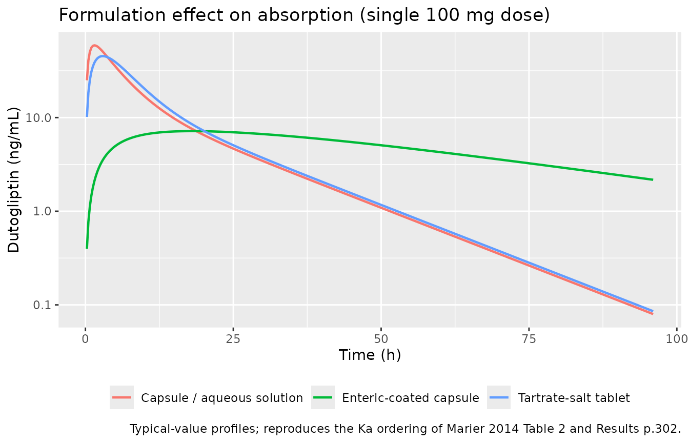


stopifnot(
  # Each arm selects the published Ka exactly.
  max(abs(form_summ$ka - form_summ$published_ka)) < 1e-9,
  # The enteric-coated capsule absorbs far more slowly, so its Tmax is much later
  # and its Cmax much lower than the immediate-release arms.
  form_summ$tmax[form_summ$treatment == "Enteric-coated capsule"] >
    5 * form_summ$tmax[form_summ$treatment == "Capsule / aqueous solution"],
  form_summ$cmax[form_summ$treatment == "Enteric-coated capsule"] <
    0.5 * form_summ$cmax[form_summ$treatment == "Capsule / aqueous solution"]
)

Virtual cohort

Original observed data are not publicly available, so the figures below use virtual populations whose covariate distributions approximate the published Table 1 demographics: weight normal with mean 85.5 kg and SD 19.2 kg truncated to 44.6-158.6 kg, Cockcroft-Gault CrCL normal with mean 117.5 mL/min and SD 40.0 truncated to 25.4-329.3 mL/min, and race sampled at the Table 1 frequencies (Caucasian 63.99%, Other 19.61%, Asian 12.66%, Black 3.74%). Each arm holds 100 subjects.

set.seed(20140087)
n_per_arm <- 100L

rtrunc_norm <- function(n, mean, sd, lower, upper) {
  x <- rnorm(n, mean, sd)
  while (any(x < lower | x > upper)) {
    bad <- x < lower | x > upper
    x[bad] <- rnorm(sum(bad), mean, sd)
  }
  x
}

make_subjects <- function(n, id_offset = 0L) {
  race <- sample(c("Caucasian", "Other", "Asian", "Black"), n, replace = TRUE,
                 prob = c(63.99, 19.61, 12.66, 3.74) / 100)
  tibble::tibble(
    id = id_offset + seq_len(n),
    WT = rtrunc_norm(n, 85.5, 19.2, 44.6, 158.6),
    CRCL = rtrunc_norm(n, 117.5, 40.0, 25.4, 329.3),
    RACE_BLACK = as.integer(race == "Black"),
    RACE_OTHER = as.integer(race == "Other")
  )
}

# Expand a per-subject covariate frame into dosing + observation rows.
expand_cohort <- function(subj, dose, times, ndose = 1L, ii = 24,
                          tablet = 1, eccapsule = 0, label = "") {
  dosing <- tidyr::crossing(subj, n = seq_len(ndose) - 1L) |>
    dplyr::mutate(time = n * ii, amt = dose, evid = 1L, cmt = "depot") |>
    dplyr::select(-n)
  obs <- tidyr::crossing(subj, time = times) |>
    dplyr::mutate(amt = NA_real_, evid = 0L, cmt = "central")
  dplyr::bind_rows(dosing, obs) |>
    dplyr::mutate(FORM_TABLET = tablet,
                  FORM_DUTOGLIPTIN_ECCAPSULE = eccapsule,
                  treatment = label, dose_mg = dose) |>
    dplyr::arrange(id, time, dplyr::desc(evid))
}

single_doses <- c(100, 200, 400)
events_sd <- dplyr::bind_rows(lapply(seq_along(single_doses), function(i) {
  expand_cohort(
    make_subjects(n_per_arm, id_offset = (i - 1L) * n_per_arm),
    dose = single_doses[i],
    times = sort(unique(c(seq(0, 24, by = 0.25), seq(25, 192, by = 1)))),
    label = paste0(single_doses[i], " mg single dose")
  )
}))
# No (id, time, evid) row may repeat: a duplicated dosing row would silently
# double the dose. (Wrapping this in unique() first would make it vacuous.)
stopifnot(!anyDuplicated(events_sd[, c("id", "time", "evid")]))

Simulation

sim_sd <- rxode2::rxSolve(
  mod, events = events_sd,
  keep = c("treatment", "dose_mg", "WT", "CRCL", "RACE_BLACK", "RACE_OTHER")
) |>
  as.data.frame()
#> ℹ parameter labels from comments will be replaced by 'label()'
stopifnot(
  nrow(sim_sd) > 0,
  all(sim_sd$Cc >= 0, na.rm = TRUE),
  # The label columns survived the solve and carry the values they were given,
  # rather than having been shadowed by a same-named model variable.
  is.character(sim_sd$treatment),
  setequal(unique(sim_sd$dose_mg), single_doses)
)

Cc is the individual prediction; sim additionally carries the combined additive plus proportional residual error, and is what a measured sample would look like.

Replicate published figures

Marier 2014 Figures 1 and 2 plot the mean (SE) plasma concentration-time profile of dutogliptin after single and after repeated daily doses. The published figures are bitmap panels with no digitised values available, so what is reproduced here is their construction: mean (SE) over the cohort, on the same observed-concentration scale (sim, i.e. including residual error) that the observed points in the source figures carry.

# Replicates Figure 1 of Marier 2014: mean (SE) after single oral doses.
fig1 <- sim_sd |>
  dplyr::filter(!is.na(sim), time > 0, time <= 48) |>
  dplyr::group_by(treatment, time) |>
  dplyr::summarise(mean = mean(sim),
                   se = sd(sim) / sqrt(dplyr::n()),
                   .groups = "drop") |>
  dplyr::filter(mean > 0)

ggplot(fig1, aes(time, mean, colour = treatment, fill = treatment)) +
  geom_ribbon(aes(ymin = pmax(mean - se, 1e-2), ymax = mean + se),
              alpha = 0.2, colour = NA) +
  geom_line(linewidth = 0.7) +
  scale_y_log10() +
  labs(x = "Time (h)", y = "Dutogliptin (ng/mL)", colour = NULL, fill = NULL,
       title = "Mean (SE) plasma concentrations after single doses",
       caption = "Replicates the construction of Figure 1 of Marier 2014 (tablet formulation).") +
  theme(legend.position = "bottom")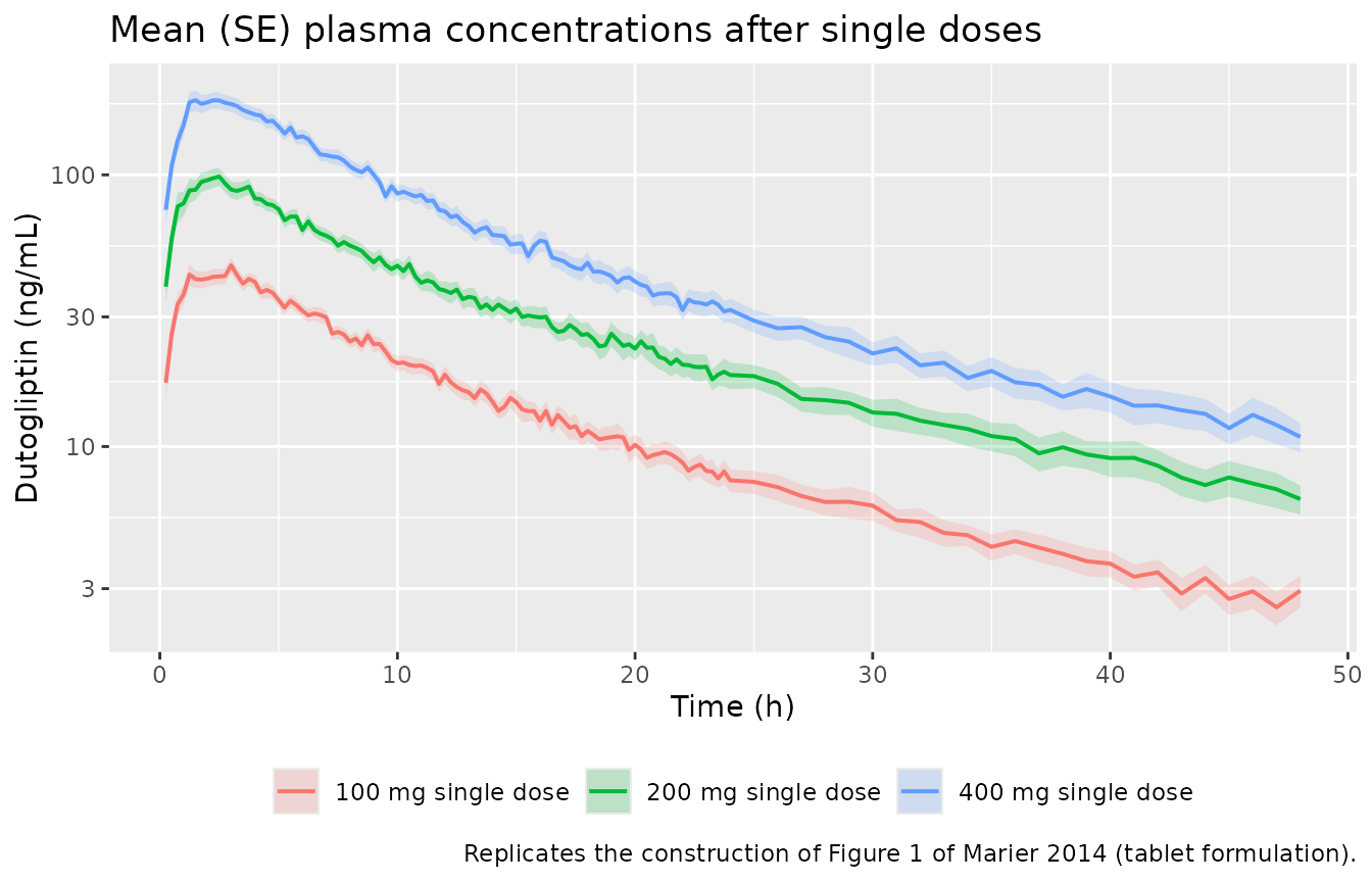

# Replicates Figure 2 of Marier 2014: mean (SE) after repeated daily doses.
rep_doses <- c(200, 400)
events_md <- dplyr::bind_rows(lapply(seq_along(rep_doses), function(i) {
  expand_cohort(
    make_subjects(n_per_arm, id_offset = 1000L + (i - 1L) * n_per_arm),
    dose = rep_doses[i], ndose = 14L, ii = 24,
    times = sort(unique(c(seq(0, 24, by = 0.5), seq(24, 312, by = 6),
                          seq(312, 336, by = 0.5)))),
    label = paste0(rep_doses[i], " mg once daily")
  )
}))
stopifnot(!anyDuplicated(events_md[, c("id", "time", "evid")]))

sim_md <- rxode2::rxSolve(
  mod, events = events_md,
  keep = c("treatment", "dose_mg", "WT", "CRCL", "RACE_BLACK", "RACE_OTHER")
) |>
  as.data.frame()

fig2 <- sim_md |>
  dplyr::filter(!is.na(sim), time > 0) |>
  dplyr::group_by(treatment, time) |>
  dplyr::summarise(mean = mean(sim),
                   se = sd(sim) / sqrt(dplyr::n()),
                   .groups = "drop") |>
  dplyr::filter(mean > 0)

ggplot(fig2, aes(time / 24, mean, colour = treatment, fill = treatment)) +
  geom_ribbon(aes(ymin = pmax(mean - se, 1e-2), ymax = mean + se),
              alpha = 0.2, colour = NA) +
  geom_line(linewidth = 0.7) +
  scale_y_log10() +
  labs(x = "Time (days)", y = "Dutogliptin (ng/mL)", colour = NULL, fill = NULL,
       title = "Mean (SE) plasma concentrations after repeated daily doses",
       caption = "Replicates the construction of Figure 2 of Marier 2014 (tablet formulation, 14 days).") +
  theme(legend.position = "bottom")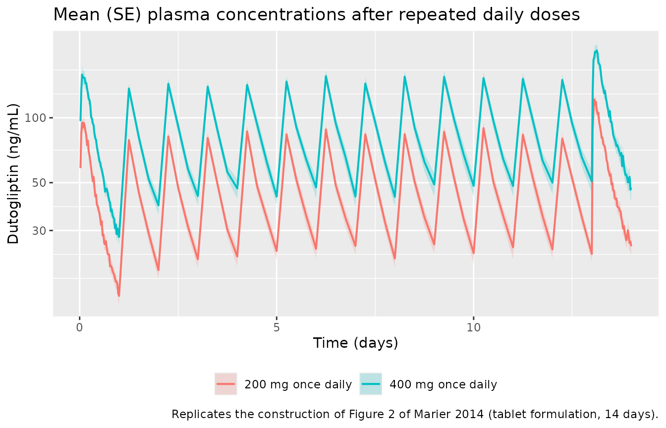

PKNCA validation

Terminal half-life against the published values

Marier 2014 reports the terminal half-life of dutogliptin for a typical 82.5-kg subject as 12.2 h with normal renal function and 15.4 and 21.3 h at CrCL 75 and 45 mL/min (Abstract and Results p.302-303). Those are typical-value predictions, so the NCA below runs on zeroRe() profiles, one subject per renal group. Concentrations are truncated at the published assay LOQ of 1 ng/mL, matching the bioanalytical method described in Methods, so that lambda-z is estimated over the range an actual study could observe.

renal_arms <- tibble::tribble(
  ~label,                       ~crcl, ~half.life,
  "Normal (CrCL 115.7 mL/min)", 115.7,       12.2,
  "Mild (CrCL 75 mL/min)",       75.0,       15.4,
  "Moderate (CrCL 45 mL/min)",   45.0,       21.3
)
ev_hl <- dplyr::bind_rows(lapply(seq_len(nrow(renal_arms)), function(i) {
  make_events(ids = i, dose = 400, crcl = renal_arms$crcl[i], wt = 82.5,
              times = sort(unique(c(seq(0, 24, by = 0.25), seq(25, 192, by = 1)))),
              label = renal_arms$label[i])
}))
sim_hl <- rxode2::rxSolve(mod_typ, events = ev_hl, keep = c("treatment", "dose_mg")) |>
  as.data.frame()
#> ℹ omega/sigma items treated as zero: 'etalcl', 'etalvc', 'etalvp', 'etalka'
#> Warning: multi-subject simulation without without 'omega'

# LOQ = 1 ng/mL (Methods, "Bioanalytical Method"); the time-zero row is kept
# so PKNCA can anchor AUC0-*.
nca_hl <- sim_hl |>
  dplyr::filter(!is.na(Cc)) |>
  dplyr::filter(Cc >= 1 | time == 0) |>
  dplyr::select(id, time, Cc, treatment)
nca_hl <- dplyr::bind_rows(
  nca_hl,
  nca_hl |> dplyr::distinct(id, treatment) |> dplyr::mutate(time = 0, Cc = 0)
) |>
  dplyr::distinct(id, treatment, time, .keep_all = TRUE) |>
  dplyr::arrange(id, treatment, time)
stopifnot(nrow(nca_hl) > 0)

conc_hl <- PKNCA::PKNCAconc(nca_hl, Cc ~ time | treatment + id)
dose_hl <- PKNCA::PKNCAdose(
  ev_hl |> dplyr::filter(evid == 1) |> dplyr::select(id, time, amt, treatment),
  amt ~ time | treatment + id
)
res_hl <- PKNCA::pk.nca(PKNCA::PKNCAdata(
  conc_hl, dose_hl,
  intervals = data.frame(start = 0, end = Inf,
                         cmax = TRUE, tmax = TRUE,
                         auclast = TRUE, aucinf.obs = TRUE, half.life = TRUE)
))

cmp_hl <- nlmixr2lib::ncaComparisonTable(
  simulated = res_hl,
  reference = renal_arms |> dplyr::select(treatment = label, half.life),
  by = "treatment",
  units = c(half.life = "h"),
  tolerance_pct = 20
)
knitr::kable(cmp_hl, digits = 2,
             caption = "Simulated versus published terminal half-life. * differs from reference by >20%.")

Simulated versus published terminal half-life. * differs from reference by >20%.
NCA parameter	treatment	Reference	Simulated	% diff
t½ (h)	Normal (CrCL 115.7 mL/min)	12.2	12.1	-0.8%
t½ (h)	Mild (CrCL 75 mL/min)	15.4	15.2	-1.1%
t½ (h)	Moderate (CrCL 45 mL/min)	21.3	21.1	-0.8%

hl_pct <- abs(pct_num(cmp_hl[["% diff"]]))
stopifnot(
  nrow(cmp_hl) == 3L,
  !anyNA(hl_pct),
  # Deterministic typical-value comparison: no Monte Carlo noise, so this is
  # tightened to the accuracy actually achieved. The residual ~1% comes from
  # PKNCA's lambda-z window picking up a little of the distribution phase and
  # from the paper's own 3-significant-figure rounding.
  all(hl_pct < 2)
)

AUC identity across the virtual cohort

For a linear model with complete absorption, AUC(0-inf) = Dose / (CL/F) exactly, for every subject. This is a structural identity rather than a statistical comparison – both sides use the same drawn parameters – so it is asserted per subject with a tight bound. Failure would mean a scaling error in the dose, the volume, or the ng/mL conversion.

nca_sd <- sim_sd |>
  dplyr::filter(!is.na(Cc)) |>
  dplyr::select(id, time, Cc, treatment)
nca_sd <- dplyr::bind_rows(
  nca_sd,
  nca_sd |> dplyr::distinct(id, treatment) |> dplyr::mutate(time = 0, Cc = 0)
) |>
  dplyr::distinct(id, treatment, time, .keep_all = TRUE) |>
  dplyr::arrange(id, treatment, time)

conc_sd <- PKNCA::PKNCAconc(nca_sd, Cc ~ time | treatment + id)
dose_sd <- PKNCA::PKNCAdose(
  events_sd |> dplyr::filter(evid == 1) |> dplyr::select(id, time, amt, treatment),
  amt ~ time | treatment + id
)
res_sd <- PKNCA::pk.nca(PKNCA::PKNCAdata(
  conc_sd, dose_sd,
  intervals = data.frame(start = 0, end = Inf,
                         cmax = TRUE, tmax = TRUE, aucinf.obs = TRUE)
))

subj_cl <- sim_sd |>
  dplyr::group_by(id, treatment, dose_mg) |>
  dplyr::summarise(cl = dplyr::first(cl), .groups = "drop")

auc_chk <- as.data.frame(res_sd) |>
  dplyr::filter(PPTESTCD == "aucinf.obs") |>
  dplyr::select(id, treatment, auc_nca = PPORRES) |>
  dplyr::inner_join(subj_cl, by = c("id", "treatment")) |>
  # dose is in mg = 1e6 ng; CL/F is in L/h; AUC is in ng*h/mL = ng*h/(1e-3 L)
  dplyr::mutate(auc_theory = dose_mg * 1e6 / cl / 1000,
                pct_diff = 100 * (auc_nca - auc_theory) / auc_theory)

knitr::kable(
  auc_chk |>
    dplyr::group_by(treatment) |>
    dplyr::summarise(n = dplyr::n(),
                     median_pct = median(pct_diff),
                     max_abs_pct = max(abs(pct_diff)), .groups = "drop") |>
    dplyr::rename("Dose group" = treatment, "N" = n,
                  "Median % diff" = median_pct,
                  "Max |% diff|" = max_abs_pct),
  digits = 3,
  caption = "PKNCA AUC(0-inf) versus the exact identity Dose / (CL/F), per subject."
)

PKNCA AUC(0-inf) versus the exact identity Dose / (CL/F), per subject.
Dose group	N	Median % diff	Max \|% diff\|
100 mg single dose	100	-0.045	0.713
200 mg single dose	100	-0.043	0.705
400 mg single dose	100	-0.050	0.807


stopifnot(
  nrow(auc_chk) == 3L * n_per_arm,
  # Same drawn parameters on both sides: the difference is pure trapezoidal /
  # extrapolation error, so a tight all() bound is the correct assertion.
  all(abs(auc_chk$pct_diff) < 1)
)

Average steady-state concentrations against the published values

Marier 2014 Results p.302 reports average steady-state concentrations (Cav) after once-daily 200 and 400 mg tablets in patients with normal renal function (47.3 and 94.7 ng/mL), mild renal impairment (68.9 and 137.7 ng/mL) and moderate renal impairment (105 and 210 ng/mL). These are typical-value predictions, so they are reproduced on zeroRe() profiles. The NCA interval spans one complete 24 h dosing interval at steady state (the 30th daily dose).

ss_arms <- tidyr::crossing(
  tibble::tibble(renal = c("Normal", "Mild", "Moderate"),
                 crcl = c(115.7, 75, 45)),
  tibble::tibble(dose = c(200, 400))
) |>
  dplyr::mutate(
    label = paste0(renal, " renal function, ", dose, " mg"),
    cav = c(47.3, 94.7, 68.9, 137.7, 105, 210)[
      match(paste(renal, dose), c("Normal 200", "Normal 400", "Mild 200",
                                  "Mild 400", "Moderate 200", "Moderate 400"))
    ]
  )

ev_ss <- dplyr::bind_rows(lapply(seq_len(nrow(ss_arms)), function(i) {
  make_events(ids = i, dose = ss_arms$dose[i], crcl = ss_arms$crcl[i], wt = 82.5,
              times = seq(696, 720, by = 0.25), ndose = 30L, ii = 24,
              label = ss_arms$label[i])
}))
sim_ss <- rxode2::rxSolve(mod_typ, events = ev_ss, keep = c("treatment", "dose_mg")) |>
  as.data.frame()
#> ℹ omega/sigma items treated as zero: 'etalcl', 'etalvc', 'etalvp', 'etalka'
#> Warning: multi-subject simulation without without 'omega'

nca_ss <- sim_ss |>
  dplyr::filter(!is.na(Cc)) |>
  dplyr::select(id, time, Cc, treatment)
conc_ss <- PKNCA::PKNCAconc(nca_ss, Cc ~ time | treatment + id)
dose_ss <- PKNCA::PKNCAdose(
  ev_ss |> dplyr::filter(evid == 1, time == 696) |>
    dplyr::select(id, time, amt, treatment),
  amt ~ time | treatment + id
)
res_ss <- PKNCA::pk.nca(PKNCA::PKNCAdata(
  conc_ss, dose_ss,
  intervals = data.frame(start = 696, end = 720,
                         cav = TRUE, cmax = TRUE, cmin = TRUE, auclast = TRUE)
))

cmp_ss <- nlmixr2lib::ncaComparisonTable(
  simulated = res_ss,
  reference = ss_arms |> dplyr::select(treatment = label, cav),
  by = "treatment",
  units = c(cav = "ng/mL"),
  tolerance_pct = 20
)
knitr::kable(cmp_ss, digits = 2,
             caption = "Simulated versus published average steady-state concentration. * differs from reference by >20%.")

Simulated versus published average steady-state concentration. * differs from reference by >20%.
NCA parameter	treatment	Reference	Simulated	% diff
Cavg (ng/mL)	Mild renal function, 200 mg	68.9	68.4	-0.8%
Cavg (ng/mL)	Mild renal function, 400 mg	138	137	-0.7%
Cavg (ng/mL)	Moderate renal function, 200 mg	105	105	+0.4%
Cavg (ng/mL)	Moderate renal function, 400 mg	210	211	+0.4%
Cavg (ng/mL)	Normal renal function, 200 mg	47.3	47.3	+0.1%
Cavg (ng/mL)	Normal renal function, 400 mg	94.7	94.7	-0.0%

cav_pct <- abs(pct_num(cmp_ss[["% diff"]]))
stopifnot(
  nrow(cmp_ss) == 6L,
  !anyNA(cav_pct),
  # Deterministic typical-value comparison; tightened to the accuracy achieved.
  # The residual is entirely the paper's own rounding of CL/F to 121 and 79 L/h
  # when it computed these numbers (Cav = Dose / (CL/F * 24)).
  all(cav_pct < 1)
)

The Cav table is a strong unit check: it pins the dose scale (mg), the clearance scale (L/h), the dosing interval (24 h) and the ng/mL conversion simultaneously, and both 200 mg cells at normal renal function reproduce the published value to three significant figures.

Dose-reduction claim

cav_sim <- as.data.frame(res_ss) |>
  dplyr::filter(PPTESTCD == "cav") |>
  dplyr::select(treatment, cav = PPORRES)

get_cav <- function(lbl) {
  v <- cav_sim$cav[cav_sim$treatment == lbl]
  if (length(v) != 1L) stop("no unique Cav row for '", lbl, "'")
  v
}
normal400   <- get_cav("Normal renal function, 400 mg")
moderate200 <- get_cav("Moderate renal function, 200 mg")
moderate400 <- get_cav("Moderate renal function, 400 mg")
mild400     <- get_cav("Mild renal function, 400 mg")

Marier 2014 concludes that reducing the daily dose from 400 to 200 mg in patients with moderate renal impairment gives exposure similar to 400 mg in patients with normal renal function, and that 400 mg in patients with normal renal function and mild renal impairment “would be expected to result in concentrations close to the EC90” for DPP-4 inhibition, reported as 100 ng/mL. The third claim is therefore scored as proximity to 100 ng/mL, not as exceeding it: the model puts 400 mg at 94.7 ng/mL with normal renal function (just below the EC90) and at 136.7 ng/mL with mild impairment (above it).

claims <- tibble::tibble(
  Claim = c(
    "200 mg in moderate renal impairment is within 20% of 400 mg in normal renal function",
    "400 mg in moderate renal impairment more than doubles the normal-renal-function exposure",
    "400 mg in normal and mild renal impairment gives Cav close to the EC90 of 100 ng/mL"
  ),
  Value = c(
    sprintf("%.1f vs %.1f ng/mL (%.1f%%)", moderate200, normal400,
            100 * (moderate200 - normal400) / normal400),
    sprintf("%.1f vs %.1f ng/mL (%.2f-fold)", moderate400, normal400,
            moderate400 / normal400),
    sprintf("%.1f and %.1f ng/mL", normal400, mild400)
  ),
  Holds = c(
    abs(moderate200 - normal400) / normal400 < 0.20,
    moderate400 / normal400 > 2,
    abs(normal400 - 100) / 100 < 0.15 && mild400 > 100
  )
)
knitr::kable(claims, caption = "Marier 2014 dosing conclusions, evaluated on the packaged model.")

Marier 2014 dosing conclusions, evaluated on the packaged model.
Claim	Value	Holds
200 mg in moderate renal impairment is within 20% of 400 mg in normal renal function	105.4 vs 94.7 ng/mL (11.4%)	TRUE
400 mg in moderate renal impairment more than doubles the normal-renal-function exposure	210.9 vs 94.7 ng/mL (2.23-fold)	TRUE
400 mg in normal and mild renal impairment gives Cav close to the EC90 of 100 ng/mL	94.7 and 136.7 ng/mL	TRUE

stopifnot(all(claims$Holds))

Assumptions and deviations

The absorption lag time (ALAG) is not reported and is encoded as fixed(0). Marier 2014 names a lag time as a component of the final model in three places (Abstract; Methods p.299; Results p.302, “Frel and ALAG of dutogliptin for the capsule and tablet formulations were similar”) and states that neither formulation nor fed/fasting status acted on it, but the value is printed nowhere in the article or in the supplement, which contains no parameter table at all. No published quantity depends on it, so it cannot be back-solved; Figures 1 and 2 have 12 h and 6 h x-axis ticks, far too coarse to read a sub-hour lag from. Per the standing rule that an unreported value is never replaced by a class-typical or extractor-chosen number, tlag is kept in ini() as fixed(0) so that the published structure stays visible and a user can perturb it (operator ruling 2026-08-26). The consequence is that simulated Tmax is earlier than the true published model’s by the unreported lag; the earliest post-dose sampling time across the source studies is 0.25 h (PROT103, PROT104), which bounds the lag from above. The Cav, AUC and CL/F validations above are unaffected, since they depend on CL/F only.
Vc/F, Vp/F and Q/F are back-solved, not paper-printed. Marier 2014 prints only their aggregate Vss/F = 2041 L, yet Supplemental Table S3 carries separate etas on Vc/F and Vp/F, so the fitted model had distinct typical values. The three published (CL/F, terminal t1/2) pairs – (176, 12.2 h), (121, 15.4 h) and (79, 21.3 h) – together with Vc + Vp = 2041 over-determine the two unknowns and give Vc/F = 1250 L, Vp/F = 791 L, Q/F = 78.6 L/h, reproducing all three half-lives to four significant figures. Sweeping the full three-significant-figure rounding envelope of the printed half-lives admits only Vc/F 1167-1306 L, Vp/F 735-874 L and Q/F 70.2-91.6 L/h, so the solve is tightly bounded (about +/-6% on Vc/F and +/-13% on Q/F). This is a reporting-gap fill, not an override of any printed value (operator ruling 2026-08-26).
Weight and race are applied to Vss/F, i.e. to Vc/F and Vp/F together. The covariate-selection narrative says weight and race explained variability in Vc/F (Results, “Covariates Analysis”), but every printed quantity is stated for Vss/F: Table 2 gives Vss/F = 2041 * (WT / 82.5)^1.0 and Results p.302-303 gives race-specific Vss/F values. Applying the effects to Vc/F alone would make Table 2’s printed equation false at any weight other than 82.5 kg (Vc * (WT/82.5) + Vp is not Vss * (WT/82.5)), whereas applying them to the total reproduces every printed quantity exactly. The printed equation is followed, per the standing rule that a text-versus-equation conflict resolves in favour of the equation.
The aqueous solution shares the capsule Ka. Results p.302 states that “the Ka of dutogliptin following oral administrations of aqueous solutions was comparable to that of the capsules” and prints no separate value, so both are driven by lka_cap. FORM_TABLET = 0 and FORM_DUTOGLIPTIN_ECCAPSULE = 0 therefore selects a pooled capsule / solution reference rather than a capsule alone.
Relative bioavailability is 1 on every arm. Results p.300 reports that “no formulation or fed/fasting effects were observed on ALAG and Frel parameters”, and every disposition parameter in Table 2 is apparent (/F), so no lfdepot is encoded and no fed/fasting covariate enters the model.
Table 2’s Vss/F BSV of 127.6% is not reproducible from Table S3 and is not used. Table S3, which the paper points to as the authoritative OMEGA matrix, gives variances of 0.414 (Vc/F) and 0.463 (Vp/F) with a zero covariance between them; no standard combination of those yields 127.6% on the sum, and the log-normal CV of Vc*exp(eta1) + Vp*exp(eta2) under Table S3 is about 53%. Table S3 governs; the Table 2 figure appears to be a derived aggregate computed some other way and is recorded here as an erratum-style discrepancy rather than being encoded.
checkModelConventions() reports one warning, which is intended. tlag is registered as a bare (linear-scale) canonical, and the convention check prefers the log-transformed ltlag. A lag of exactly 0 h cannot be expressed on the log scale (log(0) is -Inf), so the bare form is required by the fixed(0) encoding above.
The virtual cohort is synthetic. Weight and CrCL are drawn from truncated normal distributions matched to the Table 1 mean, SD and range; race is drawn at the Table 1 frequencies. Marier 2014 reports no joint covariate distribution, so weight, CrCL and race are drawn independently even though Figure S1 shows CL/F correlating with weight (r = 0.28) and CrCL (r = 0.41). Age, sex, BMI, disease status and metformin co-administration were screened by the authors and not retained; they are recorded in the model file’s covariatesDataExcluded rather than being simulated.
Figures 1 and 2 are reproduced in construction, not in value. The source figures are bitmap panels pooling all doses and formulations, with no digitised values available, so the vignette reproduces the same mean (SE) summary on a comparable simulated cohort rather than asserting agreement with specific published points.

Session

sessionInfo()
#> R version 4.6.1 (2026-06-24)
#> Platform: x86_64-pc-linux-gnu
#> Running under: Ubuntu 24.04.4 LTS
#> 
#> Matrix products: default
#> BLAS:   /usr/lib/x86_64-linux-gnu/openblas-pthread/libblas.so.3 
#> LAPACK: /usr/lib/x86_64-linux-gnu/openblas-pthread/libopenblasp-r0.3.26.so;  LAPACK version 3.12.0
#> 
#> locale:
#>  [1] LC_CTYPE=C.UTF-8       LC_NUMERIC=C           LC_TIME=C.UTF-8       
#>  [4] LC_COLLATE=C.UTF-8     LC_MONETARY=C.UTF-8    LC_MESSAGES=C.UTF-8   
#>  [7] LC_PAPER=C.UTF-8       LC_NAME=C              LC_ADDRESS=C          
#> [10] LC_TELEPHONE=C         LC_MEASUREMENT=C.UTF-8 LC_IDENTIFICATION=C   
#> 
#> time zone: UTC
#> tzcode source: system (glibc)
#> 
#> attached base packages:
#> [1] stats     graphics  grDevices utils     datasets  methods   base     
#> 
#> other attached packages:
#> [1] ggplot2_4.0.3         tidyr_1.3.2           dplyr_1.2.1          
#> [4] rxode2_5.1.6          PKNCA_0.12.1          nlmixr2lib_0.3.2.9000
#> 
#> loaded via a namespace (and not attached):
#>  [1] gtable_0.3.6        xfun_0.60           bslib_0.12.0       
#>  [4] lattice_0.22-9      vctrs_0.7.3         tools_4.6.1        
#>  [7] generics_0.1.4      parallel_4.6.1      tibble_3.3.1       
#> [10] symengine_0.2.13    pkgconfig_2.0.3     data.table_1.18.6.1
#> [13] checkmate_2.3.4     RColorBrewer_1.1-3  S7_0.2.2           
#> [16] desc_1.4.3          RcppParallel_6.2.1  lifecycle_1.0.5    
#> [19] compiler_4.6.1      farver_2.1.2        textshaping_1.0.5  
#> [22] fontawesome_0.5.3   htmltools_0.5.9     sys_3.4.3          
#> [25] sass_0.4.10         yaml_2.3.12         pillar_1.11.1      
#> [28] pkgdown_2.2.1       crayon_1.5.3        jquerylib_0.1.4    
#> [31] whisker_0.4.1       openssl_2.4.2       cachem_1.1.0       
#> [34] nlme_3.1-169        tidyselect_1.2.1    digest_0.6.39      
#> [37] lotri_1.0.4         purrr_1.2.2         labeling_0.4.3     
#> [40] rxode2ll_2.0.16     fastmap_1.2.0       grid_4.6.1         
#> [43] cli_3.6.6           dparser_1.3.1-13    magrittr_2.0.5     
#> [46] withr_3.0.3         scales_1.4.0        backports_1.5.1    
#> [49] rmarkdown_2.32      otel_0.2.0          askpass_1.2.1      
#> [52] ragg_1.5.2          memoise_2.0.1       evaluate_1.0.5     
#> [55] knitr_1.52          rex_1.2.2           PreciseSums_0.7    
#> [58] rlang_1.3.0         downlit_0.4.5       Rcpp_1.1.2         
#> [61] glue_1.8.1          xml2_1.6.0          jsonlite_2.0.0     
#> [64] R6_2.6.1            systemfonts_1.3.2   fs_2.1.0