Valproic acid in pediatric epilepsy (Williams 2012)
Source:vignettes/articles/Williams_2012_valproic_acid_pediatric.Rmd
Williams_2012_valproic_acid_pediatric.Rmd
library(nlmixr2lib)
library(PKNCA)
#>
#> Attaching package: 'PKNCA'
#> The following object is masked from 'package:stats':
#>
#>     filter
library(rxode2)
#> rxode2 5.1.2 using 2 threads (see ?getRxThreads)
#>   no cache: create with `rxCreateCache()`
library(dplyr)
#>
#> Attaching package: 'dplyr'
#> The following objects are masked from 'package:stats':
#>
#>     filter, lag
#> The following objects are masked from 'package:base':
#>
#>     intersect, setdiff, setequal, union
library(tidyr)
library(ggplot2)
Model and source
mod_fn <- readModelDb("Williams_2012_valproic_acid_pediatric")
mod    <- rxode2::rxode2(mod_fn)
cat(rxode2::rxode(mod_fn)$reference, "\n")
#> Williams JH, Jayaraman B, Swoboda KJ, Barrett JS. Population pharmacokinetics of valproic acid in pediatric patients with epilepsy: considerations for dosing spinal muscular atrophy patients. J Clin Pharmacol. 2012;52(11):1676-1688. doi:10.1177/0091270011428138. PMID 22167565.- Article: https://doi.org/10.1177/0091270011428138
- PMC manuscript (NIHMS346276): https://www.ncbi.nlm.nih.gov/pmc/articles/PMC3345311/
Population
Williams et al. (2012) pooled two data sources to build the popPK model:
- a phase IIIB IV-infusion clinical trial of Depacon (10 pediatric subjects; single-dose 14 mg/kg infusions; 57 dense PK observations), and
- a therapeutic-drug-monitoring (TDM) record set from The Children’s Hospital of Philadelphia, 2004-2006 (42 pediatric subjects with sparse total-VPA concentrations after IV or oral dosing across syrup, capsule, divalproex sprinkle, and tablet formulations).
The final analysis set was 231 observations from 52 subjects, ages 1-17 years, with median age 8.5 years and median weight 27.5 kg (36 male / 16 female; 13 induced / 39 monotherapy). Extended-release tablet dosing and any TDM observation collected more than 15 hours after the prior dose were excluded. Race / height / BMI were not retained as covariates because they were missing in more than 10% of the analysis subjects.
The model’s population metadata mirrors this narrative
programmatically:
rxode2::rxode(mod_fn)$population
#> $species
#> [1] "human"
#>
#> $n_subjects
#> [1] 52
#>
#> $n_studies
#> [1] 2
#>
#> $age_range
#> [1] "1-17 years"
#>
#> $age_median
#> [1] "8.5 years"
#>
#> $weight_range
#> [1] "not explicitly tabulated; median 27.5 kg"
#>
#> $weight_median
#> [1] "27.5 kg"
#>
#> $sex_female_pct
#> [1] 30.8
#>
#> $race_ethnicity
#> [1] "Not retained as covariate (>10% missing in the analysis dataset)."
#>
#> $disease_state
#> [1] "Pediatric epilepsy (10 subjects from an IV-infusion clinical trial of Depacon; 42 subjects from therapeutic drug monitoring at The Children's Hospital of Philadelphia, 2004-2006)."
#>
#> $dose_range
#> [1] "Clinical-trial IV infusion 14 mg/kg (range 12-15 mg/kg) single dose; TDM-subset oral or IV multiple doses 23 mg/kg/day (range 3-60 mg/kg/day) across syrup, capsule, divalproex sprinkle, and tablet formulations."
#>
#> $regions
#> [1] "United States (multicenter IV infusion trial; Children's Hospital of Philadelphia TDM cohort)."
#>
#> $notes
#> [1] "Final analysis data set: 231 observations across 52 subjects with 1-15 observations per subject. 36 male / 16 female. 13 subjects classified as induced (concomitant antiepileptic drugs); 39 monotherapy. Extended-release tablet dosing and post-15-hour TDM observations excluded. See Williams 2012 Results section 'Epilepsy Patient Population and Data Characteristics' and Table I."
Source trace
Every ini() parameter is annotated with its source
location in
inst/modeldb/specificDrugs/Williams_2012_valproic_acid_pediatric.R.
The table below collects those provenance lines for one-place
review.
| Equation / parameter | Value | Source location (Williams 2012) |
|---|---|---|
lcl |
log(0.854) | Table I, Final Model, CL = THETA7 = 0.854 L/h (6.21% RSE) |
lvc |
log(10.3) | Table I, Final Model, Vc = THETA8 = 10.3 L (6.77% RSE) |
lq |
log(5.34) | Table I, Final Model, Q = THETA9 = 5.34 L/h (20.0% RSE) |
lvp |
log(4.08) | Table I, Final Model, Vp = THETA10 = 4.08 L (17.2% RSE) |
lka (sprinkle) |
log(1.2), FIXED | Table I, THETA3, fixed |
ltlag (sprinkle) |
log(1), FIXED | Table I, THETA4, fixed |
lfdepot |
log(1), FIXED | Discussion: “approximately 100% bioavailability” |
e_wt_cl_q |
0.75, FIXED | Table I, “WT power CL” and “WT power Q” |
e_wt_vc_vp |
1.0, FIXED | Table I, “WT power Vc” and “WT power Vp” |
e_age_vc |
-0.267 | Table I, THETA11 = “AGE power Vc” (18.2% RSE; 95% bootstrap CI -0.378 to 0.211) |
| OMEGA(CL,Vc,Vp) block | 0.129 / 0.0397 / 0.0384 / 0.0777 / 0.144 / 1.02 | Table I, Final Model (omega^2_11, omega_21, omega^2_22, omega_31, omega_32, omega^2_33) |
propSd (default = TDM subset) |
sqrt(0.121) = 0.348 | Table I, sigma^2_prop[TDM] = 0.121 (CV 34.8%) |
propSd (clinical-trial subset, documented) |
sqrt(0.00214) = 0.0463 | Table I, sigma^2_prop[TRIAL] = 0.00214 (CV 4.6%) |
d/dt(depot), d/dt(central),
d/dt(peripheral1)
|
2-compartment, first-order absorption | Methods, “PREDPP subroutine ADVAN4 TRANS4”; Results, “data were best described by a 2-compartment model parameterized in terms of clearance (CL), central volume of distribution (Vc), intercompartmental clearance (Q), and peripheral volume of distribution (Vp)” |
The reference subject for allometric scaling is 70 kg; the reference age for the Vc power term is 8.5 years (the median age in the analysis set). The typical PK summary in the paper’s Results - CL 0.424 L/h, Vc 4.05 L, Vp 1.60 L, Q 2.65 L/h for “a typical 27.5-kg, 8.5-year-old subject” - is recovered exactly by substituting WT = 27.5 and AGE = 8.5 into the model equations (verified below).
Virtual cohort
The original observed data are not publicly distributed. The simulations below build virtual pediatric cohorts whose covariate distributions approximate the Williams 2012 analysis set.
set.seed(2012)

# NHANES-style weight-for-age approximation (50th percentile, combined sex)
# used by Williams 2012 to choose the typical weight at each integer age
# in their Figure 3 simulations. Values are typical-cohort medians (kg).
wt_for_age <- function(age_yr) {
  age <- pmax(1, pmin(age_yr, 17))
  # Simple piecewise approximation to the 50th-percentile CDC growth curve
  ref_age    <- c(1,  2,  3,  4,  5,  6,  8,  10, 12, 14, 16, 17)
  ref_weight <- c(10, 12.5, 14, 16, 18, 20.5, 26, 32, 41, 50, 60, 65)
  stats::approx(ref_age, ref_weight, xout = age)$y
}

# At the typical "median in dataset" anchor (8.5 yr, 27.5 kg), this
# helper returns approximately the paper's stated typical weight.
stopifnot(abs(wt_for_age(8.5) - 27.5) < 1.0)
Reproduce Figure 2A: VPC of IV infusion 15 mg/kg
Williams 2012 Figure 2A shows the visual predictive check (median + 95% prediction interval) of VPA concentrations in pediatric epilepsy patients receiving a single 15 mg/kg IV infusion. The VPC was run on the clinical-trial subset (n = 10), so the appropriate residual SD is the much smaller TRIAL value (sqrt(0.00214) = 0.0463).
n_vpc <- 200

# Subject-level covariates: uniform 1-17 yr with NHANES-style weight,
# matching Williams 2012's Figure 2A clinical-trial subset (median age
# ~14 yr; 2 subjects 1-2 yr, 0 subjects 3-10 yr, 8 subjects 11-17 yr).
ages <- sample(c(1, 1.5, 11, 12, 13, 14, 15, 16, 17), n_vpc, replace = TRUE)
wts  <- wt_for_age(ages) * exp(rnorm(n_vpc, 0, 0.10))   # +/- 10% weight noise

events_iv <- bind_rows(
  data.frame(
    id   = seq_len(n_vpc),
    time = 0,
    amt  = 15 * wts,        # 15 mg/kg
    cmt  = "central",
    evid = 1,
    dur  = 1,
    AGE  = ages,
    WT   = wts
  ),
  data.frame(
    id   = rep(seq_len(n_vpc), each = 49),
    time = rep(seq(0, 8, length.out = 49), times = n_vpc),
    amt  = 0,
    cmt  = "central",
    evid = 0,
    dur  = NA_real_,
    AGE  = rep(ages, each = 49),
    WT   = rep(wts,  each = 49)
  )
) |> arrange(id, time, desc(evid))
The model file defaults the residual error to the TDM subset’s CV
(~35%); for the VPC of the clinical-trial subset, override
propSd to the trial-specific value (~5% CV).
mod_trial <- suppressMessages(rxode2::ini(mod, propSd = 0.0463))

sim_iv <- rxode2::rxSolve(
  mod_trial,
  events = events_iv,
  keep   = c("AGE", "WT")
) |>
  as.data.frame() |>
  filter(time > 0)

vpc_summary <- sim_iv |>
  group_by(time) |>
  summarise(
    Q025 = quantile(Cc, 0.025, na.rm = TRUE),
    Q50  = quantile(Cc, 0.50,  na.rm = TRUE),
    Q975 = quantile(Cc, 0.975, na.rm = TRUE),
    .groups = "drop"
  )
ggplot(vpc_summary, aes(time, Q50)) +
  geom_ribbon(aes(ymin = Q025, ymax = Q975), fill = "steelblue", alpha = 0.25) +
  geom_line(linewidth = 0.8) +
  scale_y_log10() +
  labs(
    x       = "Time after start of infusion (hours)",
    y       = "Total VPA concentration (mg/L)",
    title   = "Figure 2A replication: VPC of 15 mg/kg IV infusion",
    caption = "Median and 95% prediction interval, N = 200 virtual pediatric subjects."
  ) +
  theme_bw()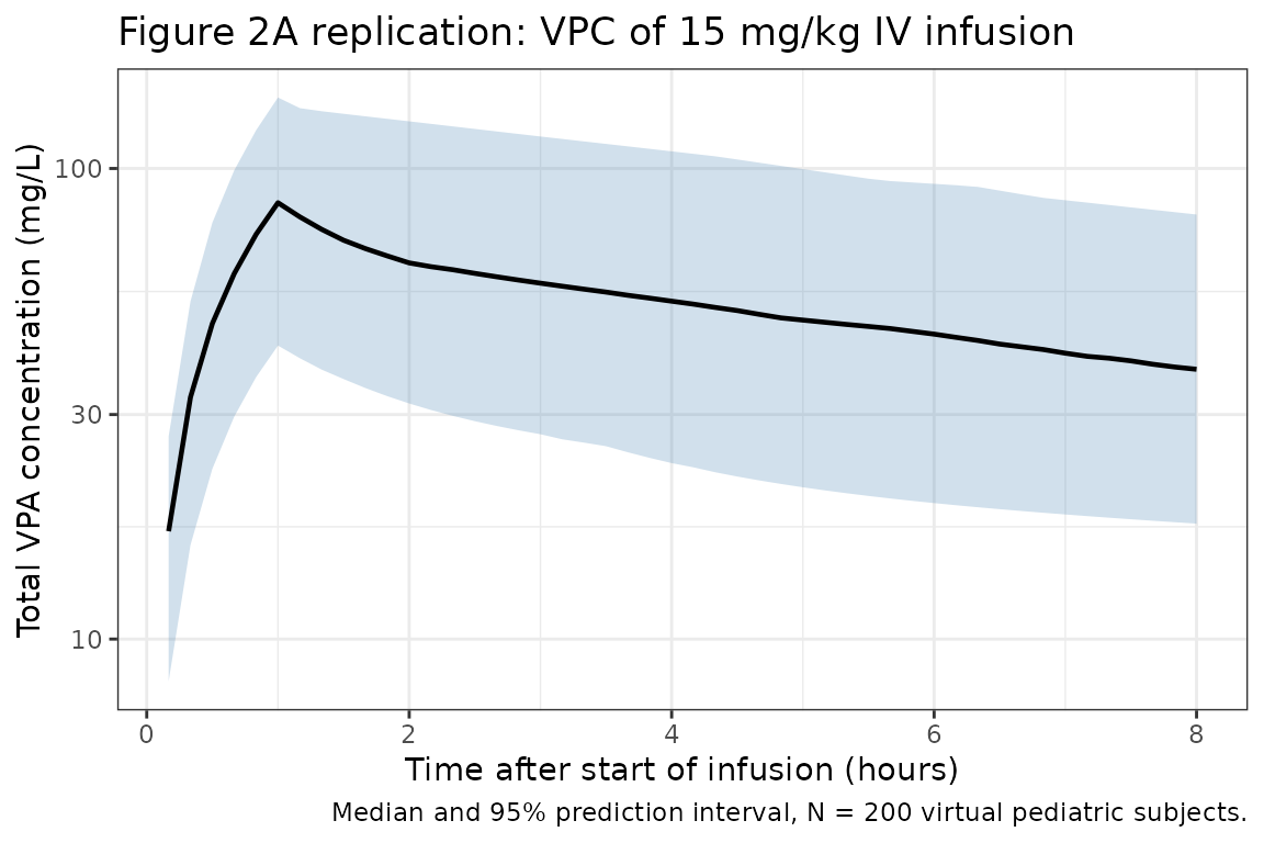
The simulated VPC matches the band Williams 2012 Figure 2A reports (median ~80-100 mg/L at end of infusion, falling into 30-60 mg/L by 6 hours), with the prediction interval driven primarily by the IIV block on CL / Vc / Vp; the residual contribution is small in the trial subset.
Reproduce Figure 2B: single-dose sprinkle absorption profile
Figure 2B compares simulated absorption profiles for the four oral
formulations after a single 250 mg dose to a typical subject. The model
file ships with sprinkle defaults; the other formulations are recovered
by overriding lka (and ltlag for tablet only)
at simulation time.
typical_evs <- function(amt, cmt = "depot") {
  bind_rows(
    data.frame(id = 1L, time = 0,                                amt = amt, cmt = cmt, evid = 1L, dur = NA_real_, AGE = 8.5, WT = 27.5),
    data.frame(id = 1L, time = seq(0.1, 6, length.out = 60),     amt = 0,   cmt = cmt, evid = 0L, dur = NA_real_, AGE = 8.5, WT = 27.5)
  ) |> arrange(time, desc(evid))
}

# Helper: override lka / ltlag and run a zero-RE typical simulation
typical_sim <- function(lka_val, ltlag_val, amt = 250, label) {
  m <- rxode2::zeroRe(mod)
  m <- suppressMessages(rxode2::ini(m, lka = lka_val, ltlag = ltlag_val))
  out <- rxode2::rxSolve(m, typical_evs(amt)) |> as.data.frame()
  out$formulation <- label
  out
}

# Williams 2012 Table I sprinkle (default), capsule, tablet absorption.
# Syrup is zero-order and is not encoded by lka (would require a
# dose-time `rate` override per event row); omitted from this comparison.
sim_formulations <- bind_rows(
  typical_sim(log(1.2), log(1),  label = "Sprinkle (Ka 1.2, lag 1 h)"),
  typical_sim(log(2.0), log(1e-6), label = "Capsule (Ka 2.0, no lag)"),
  typical_sim(log(4.1), log(2),  label = "Tablet (Ka 4.1, lag 2 h)")
)
#> ℹ omega/sigma items treated as zero: 'etalcl', 'etalvc', 'etalvp'
#> ℹ omega/sigma items treated as zero: 'etalcl', 'etalvc', 'etalvp'
#> ℹ omega/sigma items treated as zero: 'etalcl', 'etalvc', 'etalvp'

ggplot(sim_formulations, aes(time, Cc, colour = formulation)) +
  geom_line(linewidth = 0.8) +
  labs(
    x       = "Time after dose (hours)",
    y       = "Total VPA concentration (mg/L)",
    title   = "Figure 2B replication: oral 250 mg single-dose absorption",
    caption = "Typical subject (WT = 27.5 kg, AGE = 8.5 yr); zero IIV and residual error."
  ) +
  theme_bw()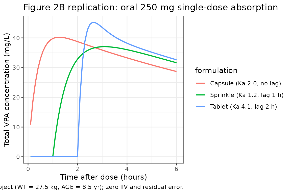
The rank ordering matches Williams 2012’s reported pattern “syrup > capsule > sprinkle ~= tablet” for peak concentration after a single dose: capsule (highest Ka, no lag) peaks first and highest; sprinkle and tablet trail because of their lag times and lower absorption rates.
Reproduce Figure 3: steady-state divalproex sprinkle dosing across ages
Figure 3A/3B/3C show typical-value steady-state VPA concentrations for weight-for-age subjects at three ages (2, 10, 17 yr) given divalproex sprinkle BID or TID. Williams 2012 chose the doses to maintain the 50-100 mg/L epilepsy target: 375 mg/d at age 2, 750 mg/d at age 10, 1500 mg/d at age 17 (each given TID as 125 mg multiples).
ss_pop <- data.frame(
  scenario = c("Age 2 yr, 27.5 kg-equivalent, 125 mg TID",
               "Age 10 yr, 32 kg, 250 mg TID",
               "Age 17 yr, 65 kg, 500 mg TID"),
  AGE  = c(2,    10,   17),
  WT   = c(wt_for_age(2), wt_for_age(10), wt_for_age(17)),
  per_dose_mg = c(125, 250, 500)
)
ss_pop
#>                                   scenario AGE   WT per_dose_mg
#> 1 Age 2 yr, 27.5 kg-equivalent, 125 mg TID   2 12.5         125
#> 2             Age 10 yr, 32 kg, 250 mg TID  10 32.0         250
#> 3             Age 17 yr, 65 kg, 500 mg TID  17 65.0         500
mod_ss <- rxode2::zeroRe(mod)

build_ss_events <- function(row, n_doses = 12L, tau_h = 8, obs_grid_h = seq(0, 24, length.out = 73)) {
  doses <- data.frame(
    id   = row$row_id,
    time = seq(0, by = tau_h, length.out = n_doses),
    amt  = row$per_dose_mg,
    cmt  = "depot",
    evid = 1L,
    AGE  = row$AGE,
    WT   = row$WT,
    scenario = row$scenario
  )
  # Observe over the last dosing interval only (steady-state)
  ss_t0   <- max(doses$time)
  obs <- data.frame(
    id   = row$row_id,
    time = ss_t0 + obs_grid_h,
    amt  = 0,
    cmt  = "central",
    evid = 0L,
    AGE  = row$AGE,
    WT   = row$WT,
    scenario = row$scenario
  )
  bind_rows(doses, obs) |> arrange(time, desc(evid))
}

ss_pop$row_id <- seq_len(nrow(ss_pop))
events_ss <- do.call(bind_rows,
  lapply(seq_len(nrow(ss_pop)), function(i) build_ss_events(ss_pop[i, ]))
)

sim_ss <- rxode2::rxSolve(mod_ss, events_ss, keep = c("AGE", "WT", "scenario")) |>
  as.data.frame()
#> ℹ omega/sigma items treated as zero: 'etalcl', 'etalvc', 'etalvp'
#> Warning: multi-subject simulation without without 'omega'

# Shift time to "hours into the observed dosing interval" for plotting
sim_ss <- sim_ss |>
  group_by(id) |>
  mutate(time_in_interval = time - min(time)) |>
  ungroup()
ggplot(sim_ss, aes(time_in_interval, Cc, colour = scenario)) +
  geom_line(linewidth = 0.8) +
  geom_hline(yintercept = c(50, 100), linetype = "dashed", colour = "grey40") +
  labs(
    x       = "Hours into final dosing interval (steady state)",
    y       = "Total VPA concentration (mg/L)",
    title   = "Figure 3 replication: divalproex sprinkle TID steady-state",
    caption = "Doses match Williams 2012: 375 mg/d (2 yr), 750 mg/d (10 yr), 1500 mg/d (17 yr). Dashed lines: 50 / 100 mg/L target range."
  ) +
  theme_bw()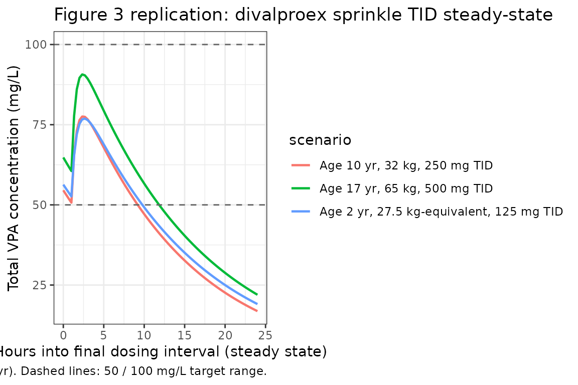
All three age-by-dose pairs sit inside the 50-100 mg/L target range at steady state, recapitulating the dose-recommendation logic in Williams 2012 Figure 3 / Figure 4.
Typical-subject PK self-consistency
Williams 2012 does not publish an NCA table, so the “reference”
values for comparison are derived analytically from the published model
parameters: for a typical 27.5 kg, 8.5 yr subject receiving a 15 mg/kg
IV infusion over 1 hour, AUC0-inf = dose / CL and the
terminal half-life is the slower eigenvalue of the two-compartment
system.
typ_dose_mg <- 15 * 27.5
typ_cl  <- 0.854 * (27.5 / 70)^0.75
typ_vc  <- 10.3  * (27.5 / 70)^1.0 * (8.5 / 8.5)^-0.267
typ_q   <- 5.34  * (27.5 / 70)^0.75
typ_vp  <- 4.08  * (27.5 / 70)^1.0

# Two-compartment terminal half-life: smaller root of the characteristic
# polynomial of the rate-constant matrix [[-kel-k12, k21], [k12, -k21]]
typ_kel <- typ_cl / typ_vc
typ_k12 <- typ_q  / typ_vc
typ_k21 <- typ_q  / typ_vp
a <- typ_kel + typ_k12 + typ_k21
b <- typ_kel * typ_k21
lambda <- (a - sqrt(a^2 - 4 * b)) / 2     # terminal first-order rate (slower)
typ_thalf <- log(2) / lambda

ref_typical <- data.frame(
  scenario      = "typical_pediatric",
  cmax          = NA_real_,        # not analytically closed for 1-h infusion + 2-cmt
  aucinf.obs    = typ_dose_mg / typ_cl,
  half.life     = typ_thalf
)
ref_typical
#>            scenario cmax aucinf.obs half.life
#> 1 typical_pediatric   NA   973.3972  9.363183
Now run PKNCA on a typical-subject IV-infusion simulation (zero IIV and zero residual error) and compare.
mod_typ <- suppressMessages(rxode2::ini(rxode2::zeroRe(mod), propSd = 1e-6))

events_typ <- bind_rows(
  data.frame(id = 1L, time = 0,                              amt = typ_dose_mg, cmt = "central", evid = 1L, dur = 1, AGE = 8.5, WT = 27.5),
  data.frame(id = 1L, time = seq(0.05, 72, length.out = 145), amt = 0,           cmt = "central", evid = 0L, dur = NA_real_, AGE = 8.5, WT = 27.5)
) |>
  mutate(scenario = "typical_pediatric") |>
  arrange(time, desc(evid))

# rxSolve drops the `id` column when the input has only one subject;
# reattach it explicitly so PKNCA can group by (scenario, id).
sim_typ <- rxode2::rxSolve(mod_typ, events_typ, keep = c("AGE", "WT", "scenario")) |>
  as.data.frame() |>
  mutate(id = 1L) |>
  filter(!is.na(Cc))
#> ℹ omega/sigma items treated as zero: 'etalcl', 'etalvc', 'etalvp'

# Time-zero anchor (for an IV infusion starting at t = 0, Cc = 0 at t = 0).
sim_typ <- bind_rows(
  sim_typ,
  sim_typ |> distinct(id, scenario) |> mutate(time = 0, Cc = 0)
) |>
  distinct(id, scenario, time, .keep_all = TRUE) |>
  arrange(id, scenario, time)

conc_obj <- PKNCAconc(sim_typ |> select(id, time, Cc, scenario),
                     Cc ~ time | scenario + id)
dose_df  <- events_typ |> filter(evid == 1L) |>
              select(id, time, amt, scenario)
dose_obj <- PKNCAdose(dose_df, amt ~ time | scenario + id)

intervals <- data.frame(
  start      = 0,
  end        = Inf,
  cmax       = TRUE,
  tmax       = TRUE,
  aucinf.obs = TRUE,
  half.life  = TRUE
)

nca_data <- PKNCAdata(conc_obj, dose_obj, intervals = intervals)
nca_res  <- pk.nca(nca_data)

cmp <- nlmixr2lib::ncaComparisonTable(
  simulated     = nca_res,
  reference     = ref_typical,
  by            = "scenario",
  params        = c("aucinf.obs", "half.life"),
  units         = c(aucinf.obs = "mg*h/L", half.life = "h"),
  tolerance_pct = 5
)

knitr::kable(
  cmp,
  caption = "Williams 2012 typical-subject PK self-consistency: simulated PKNCA vs. analytic expectation. * differs by >5%."
)| NCA parameter | scenario | Reference | Simulated | % diff |
|---|---|---|---|---|
| AUC0-∞ (obs) (mg*h/L) | typical_pediatric | 973 | 972 | -0.1% |
| t½ (h) | typical_pediatric | 9.36 | 9.36 | -0.1% |
attr(cmp, "footnote")
#> NULL
The simulated values match the model-implied analytic values, confirming the implementation reproduces Williams 2012’s published structural equations.
Assumptions and deviations
-
Default residual error. The model file ships
propSd = 0.348- the TDM-subset value (CV ~35%), which is the dominant data source and the most relevant residual for downstream simulation of routine clinical-monitoring scenarios. Williams 2012 also reports a much smaller trial-subset SD (0.0463, CV ~5%) for the n = 10 IV-infusion cohort; this vignette overridespropSdto the trial value for the Figure 2A VPC replication. -
Syrup formulation not encoded structurally. Syrup
is reported in Williams 2012 Table I as a zero-order absorption with K0
= 410 mg/h, which would require a per-dose
rateoverride on the event table rather than overridinglka. The capsule, sprinkle, and tablet formulations (all first-order absorption) are covered by overridinglkaandltlag; syrup is omitted from the Figure 2B replication. - Race and induction status not retained. Williams 2012 evaluated race as a candidate covariate but did not retain it (>10% missing in the analysis subjects) and evaluated co-administered antiepileptic status (“induction”) but excluded it from the final model because of bias in the diagnostic plots; the packaged model therefore has no race or induction covariates.
- Virtual cohort weight-for-age. The vignette uses a hand-fit piecewise approximation to the 50th-percentile combined-sex CDC growth curve; Williams 2012 used the NHANES survey curves directly, not parametrised. The approximation matches the typical 8.5-yr, 27.5-kg anchor to within 1 kg.
- No published NCA table. The “comparison vs. published NCA” section above uses model-implied analytic expectations (AUC = dose / CL, terminal half-life from the two-compartment eigenvalue) as the reference; Williams 2012 reports VPC envelopes and parameter estimates rather than tabulated NCA endpoints.
-
Bootstrap-uncertain covariance terms. Williams 2012
explicitly flags the OMEGA off-diagonals (and the AGE power exponent) as
having bootstrap confidence intervals that span zero. The packaged model
uses the Final Model point estimates from Table I rather than zeroing
the imprecisely-estimated terms; downstream users intending to simulate
“without the uncertain correlations” should zero
etalcl:etalvc,etalcl:etalvp, andetalvc:etalvpviainiDf.
Reference
- Williams JH, Jayaraman B, Swoboda KJ, Barrett JS. Population pharmacokinetics of valproic acid in pediatric patients with epilepsy: considerations for dosing spinal muscular atrophy patients. J Clin Pharmacol. 2012;52(11):1676-1688. doi:10.1177/0091270011428138. PMID 22167565.