Contezolid acefosamil and contezolid (Bulitta 2024)
Source:vignettes/articles/Bulitta_2024_contezolid.Rmd
Bulitta_2024_contezolid.RmdModel and source
- Citation: Bulitta JB, Fang E, Stryjewski ME, Wang W, Atiee GJ, Stark JG, Hafkin B. Population pharmacokinetic rationale for intravenous contezolid acefosamil followed by oral contezolid dosage regimens. Antimicrob Agents Chemother. 2024;68(4):e01400-23. doi:10.1128/aac.01400-23. Preliminary results presented as Bulitta JB, Hafkin B, Fang E. 1118. Population Pharmacokinetics of Contezolid Acefosamil and Contezolid - Rationale for a Safe and Effective Loading Dose Regimen. Open Forum Infect Dis. 2021;8(Suppl 1):S651. doi:10.1093/ofid/ofab466.1311.
- Description: Integrated population PK model for the intravenous double prodrug contezolid acefosamil (CZA), its intermediate MRX-1352, active contezolid and the inactive metabolite MRX-1320, jointly fitted to 110 healthy volunteers (IV CZA 150-2400 mg; oral contezolid 400-1200 mg fed/fasting) and 74 adult phase 2 patients with acute bacterial skin and skin structure infection (oral contezolid 800 mg q12h with food). CZA (amount only, not assayed) converts to MRX-1352 by Michaelis-Menten kinetics with a first-order loss; MRX-1352, contezolid and MRX-1320 each have two-compartment disposition. The MRX-1352-to-contezolid conversion clearance is auto-induced by MRX-1352 concentration (sigmoid Emax) and rises sigmoidally with time since the first dose; the MRX-1352 loss clearance shares the same auto-induction EC50 and Hill coefficient. Contezolid is converted entirely by first-order clearance to MRX-1320, which is eliminated by parallel linear and Michaelis-Menten routes. Oral contezolid passes three transit compartments (each with mean time Tlag/3) and a gut compartment with first-order absorption; lag time, absorption half-life and relative bioavailability depend on the fed state and the 400/800/1200 mg dose level. Allometric weight scaling (70 kg; exponents 0.75 clearances, 1 volumes). Separate typical contezolid clearance and between-subject variability for healthy volunteers and patients. Fitted in S-ADAPT (importance sampling).
- Article: https://doi.org/10.1128/aac.01400-23
- Preliminary conference abstract (IDWeek 2021 poster 1118): https://doi.org/10.1093/ofid/ofab466.1311
The 2021 abstract reported an earlier cut of the same analysis (for example an apparent contezolid clearance of 13.1 L/h in healthy volunteers and a steady-state volume of 20.5 L). Its numbers were superseded by the full paper, which is the source for every value in this model. No correction notice for the 2024 paper was found as of 2026-09-29.
Population
The model was fitted simultaneously to 184 adults from three studies (Bulitta 2024 Table 1 and Results paragraph 1):
- MRX4-002 – 66 healthy volunteers given IV contezolid acefosamil (CZA): single doses of 150 to 2400 mg over 60 or 90 min, and 600 or 900 mg q12h or 2100 mg q24h for 10 days. MRX-1352, contezolid and MRX-1320 were measured. Age 35.9 +/- 10.2 years, weight 77.9 +/- 10.0 kg; 37 Caucasian, 26 Black, 1 Asian, 2 other.
- MRX-I-02 – 44 healthy volunteers given oral contezolid: single doses of 400, 800 or 1200 mg with and without a high-fat meal (crossover), and 800 mg q12h with food for 14 or 28 days. Age 24.6 +/- 3.3 years, weight 71.2 +/- 12.7 kg; 42 Caucasian, 2 Asian.
- MRX-I-03 – 74 phase 2 patients with acute bacterial skin and skin structure infection (ABSSSI) given 800 mg oral contezolid q12h with food for 10 days, sampled at 4 and 5 h post-dose on days 3 and 7. Age 38.4 +/- 10.7 years, weight 82.8 +/- 21.7 kg; 42 Caucasian, 10 Black, 20 Hispanic, 2 other.
Across the three studies 68 of 184 subjects (37%) were female. The
same information is available programmatically via
readModelDb("Bulitta_2024_contezolid")()$population.
Model structure
The IV prodrug CZA is converted to the intermediate MRX-1352 by
Michaelis-Menten kinetics on the CZA amount (Vmax 802 mg/h,
AM50 0.96 mg), with a parallel first-order loss of CZA (half-life 19.7
min). CZA itself was not fitted (most of its concentrations were below
the quantification limit), so it is carried as an amount in
depot_iv. MRX-1352, contezolid and MRX-1320 each have
two-compartment disposition. Every conversion flux is scaled by the
product-to-substrate molecular-mass ratio (CZA 552.33, MRX-1352 487.30,
contezolid 408.33, MRX-1320 444.36 Da).
The MRX-1352 to contezolid conversion clearance has two features (Bulitta 2024 equations 1-7):
- an immediate sigmoid auto-induction by the MRX-1352
concentration,
IND = Emax * C^H / (C^H + EC50^H), which also drives the MRX-1352 loss clearance with its own maximumEmax_Lossbut the same EC50 and H; and - a time-dependent increase of the base clearance
from
CL_1352,0= 1.46 L/h toCL_1352,SS= 6.60 L/h, with half-maximal change atTC50= 116 h after the first dose.
Contezolid is converted entirely, by first-order clearance, to MRX-1320, which is eliminated by parallel linear and Michaelis-Menten routes. Oral contezolid passes three transit compartments, each with mean time Tlag/3 (Bulitta 2024 Figure 2), and a gut compartment with first-order absorption.
Source trace
Every value is from Bulitta 2024 Table 2 (‘Population mean’ and
‘Between-subject variability’ columns) unless stated otherwise. The same
origin is recorded as an in-file comment next to each ini()
entry in
inst/modeldb/specificDrugs/Bulitta_2024_contezolid.R.
| Equation / parameter | Value | Source location |
|---|---|---|
lcl / lcl_csssi (contezolid CL, healthy /
patient) |
10.2 / 11.3 L/h | Table 2, CL_Con,HV and CL_Con,PA |
lq, lvc, lvp (contezolid CLd,
V1, V2) |
69.9 L/h, 3.0 L (fixed), 14.1 L | Table 2; V1 fixed per Results |
lfdepot (F, 800 mg fed) |
0.640 | Table 2 and footnote e |
lfdepot_400fed, _400fasted,
_800fasted, _1200fed,
_1200fasted
|
0.924, 0.606, 0.467, 0.820, 0.485 | Table 2, F_rel rows (800 mg fed fixed to 1) |
lmtt / lmtt_fasted (Tlag fed /
fasting) |
47.5 / 22.5 min | Table 2; ktr = 3/Tlag from Figure 2 |
lka / lka_fasted
|
log(2)/(59.3 min), log(2)/(69.4 min) | Table 2, T_1/2,abs rows |
lvmax_cza, lkm_cza,
lkel_cza
|
802 mg/h, 0.960 mg, log(2)/(19.7 min) | Table 2, CZA rows |
lcl_mrx1352, lcl_ss_mrx1352
|
1.46, 6.60 L/h | Table 2, CL_1352,0 and CL_1352,SS; equation 4 |
lcl_t50_mrx1352,
lcl_time_hill_mrx1352
|
116 h, 2.72 | Table 2, TC_50 and Ht; equation 3 |
lemax_mrx1352, lec50_mrx1352,
lhill_mrx1352
|
145, 64.9 mg/L, 7.01 | Table 2; equations 1, 2, 5 |
lcl_loss_mrx1352, lemax_loss_mrx1352
|
0.00987 L/h, 29,400 | Table 2; equations 6, 7 |
lq_mrx1352, lvc_mrx1352,
lvp_mrx1352
|
10.2 L/h, 7.61 L, 13.0 L | Table 2 |
lcl_mrx1320, lvmax_mrx1320,
lkm_mrx1320
|
0.853 L/h, 74.2 mg/h, 0.657 mg/L | Table 2 |
lq_mrx1320, lvc_mrx1320,
lvp_mrx1320
|
16.4 L/h, 29.6 L, 67.9 L | Table 2 |
e_wt_cl, e_wt_vc
|
0.75, 1 (fixed), 70 kg | Methods, ‘Covariate effects’ |
| Between-subject variances | BSV^2 | Table 2 BSV column, footnote c |
etalvmax_mrx1320 / etalkm_mrx1320
covariance |
r = 0.949 | Table 2 footnote f |
etaiov_lfdepot_oc1, _oc2 (BOV on F) |
0.135^2 | Table 2 footnote d |
| Residual errors (six additive, six proportional terms) | see model file | Table 2 footnote h |
| Molecular masses in conversion fluxes | 552.33 / 487.30 / 408.33 / 444.36 Da | Methods, ‘Population pharmacokinetics’ |
d/dt(depot_iv) …
d/dt(peripheral1_mrx1320)
|
n/a | Figure 2 and equations 1-7 |
Simulation helpers
The paper’s Monte Carlo simulations (Methods, ‘Designing optimal IV and oral dosage regimens’) used phase 2 patients (the larger clearance variability), body weight with mean 70 kg and 20% CV, a 2000 mg CZA loading dose as a 90-min infusion at 0 h, then 1000 mg CZA over 60 min q12h, then 800 mg oral contezolid q12h with food starting 12 h after the last IV dose.
mod <- readModelDb("Bulitta_2024_contezolid")

obs_grid <- seq(0, 168, by = 0.25)

# One subject's event records for a regimen with `n_iv` IV CZA doses followed
# by oral contezolid. Observation rows sit on the contezolid `central` state
# with dvid = 1; rxSolve still returns all three endpoint columns.
make_regimen <- function(id, n_iv, t_end = 168) {
  iv_t <- c(0, 12 * seq_len(n_iv - 1))
  iv_amt <- c(2000, rep(1000, n_iv - 1))
  iv_dur <- c(1.5, rep(1, n_iv - 1))
  po_t <- 12 * n_iv + 12 * (0:100)
  po_t <- po_t[po_t < t_end]
  dplyr::bind_rows(
    data.frame(
      id = id, time = iv_t, amt = iv_amt, rate = iv_amt / iv_dur,
      cmt = "depot_iv", evid = 1L, dvid = NA_integer_
    ),
    if (length(po_t) > 0) {
      data.frame(
        id = id, time = po_t, amt = 800, rate = 0,
        cmt = "transit1", evid = 1L, dvid = NA_integer_
      )
    },
    data.frame(
      id = id, time = obs_grid[obs_grid <= t_end], amt = 0, rate = 0,
      cmt = "central", evid = 0L, dvid = 1L
    )
  )
}

# Covariates for the patient Monte Carlo cohort.
add_patient_covariates <- function(ev, wt) {
  ev |>
    dplyr::left_join(data.frame(id = seq_along(wt), WT = wt), by = "id") |>
    dplyr::mutate(
      DIS_CSSSI = 1, FED = 1, DOSE_CONTEZOLID_MG = 800,
      STUDY_MRX4002 = 0, OCC = 1
    ) |>
    dplyr::arrange(id, time, dplyr::desc(evid))
}

# Trapezoidal AUC of a finely gridded typical-value profile over [a, b].
auc_window <- function(time, conc, a, b) {
  k <- time >= a & time <= b
  x <- time[k]
  y <- conc[k]
  sum(diff(x) * (head(y, -1) + tail(y, -1)) / 2)
}
Typical-value reproduction of Table 3
Table 3 of Bulitta 2024 lists the Monte Carlo medians of daily AUCs for the three analytes. The typical patient (70 kg, all random effects at zero) is solved for each regimen and compared cell by cell. A typical-value prediction is not the median of a non-linear Monte Carlo simulation, so agreement within roughly 15% is the expectation; cells where the published median is below 5 mg*h/L (MRX-1352 after IV dosing stops) are shown but not gated.
regimens <- c("1 IV CZA dose" = 1, "4 IV CZA doses" = 4, "14 IV CZA doses" = 14)
days <- c(1, 2, 3, 4, 7)

typical <- lapply(names(regimens), function(reg) {
  ev <- make_regimen(1, regimens[[reg]]) |>
    add_patient_covariates(wt = 70)
  s <- as.data.frame(rxode2::rxSolve(mod, ev, omega = NA, sigma = NA, returnType = "data.frame"))
  do.call(rbind, lapply(days, function(d) {
    data.frame(
      regimen = reg, day = d,
      analyte = c("contezolid", "MRX-1352", "MRX-1320"),
      sim = c(
        auc_window(s$time, s$Cc, 24 * (d - 1), 24 * d),
        auc_window(s$time, s$Cc_mrx1352, 24 * (d - 1), 24 * d),
        auc_window(s$time, s$Cc_mrx1320, 24 * (d - 1), 24 * d)
      )
    )
  }))
}) |> dplyr::bind_rows()
#> ℹ parameter labels from comments will be replaced by 'label()'
#> Warning: some etas defaulted to non-mu referenced, possible parsing error: etalcl_csssi, etalfdepot_400fasted, etalfdepot_800fasted, etalfdepot_1200fed, etalfdepot_1200fasted, etalmtt_fasted, etalka_fasted, etaiov_lfdepot_oc1, etaiov_lfdepot_oc2
#> as a work-around try putting the mu-referenced expression on a simple line

# Bulitta 2024 Table 3, medians of 1,000 simulated patients (mg*h/L).
published_t3 <- tibble::tribble(
  ~regimen, ~day, ~analyte, ~published,
  "1 IV CZA dose", 1, "contezolid", 103, "1 IV CZA dose", 1, "MRX-1352", 334, "1 IV CZA dose", 1, "MRX-1320", 36.9,
  "1 IV CZA dose", 2, "contezolid", 103, "1 IV CZA dose", 2, "MRX-1352", 58.7, "1 IV CZA dose", 2, "MRX-1320", 48.3,
  "1 IV CZA dose", 3, "contezolid", 95.9, "1 IV CZA dose", 3, "MRX-1352", 7.36, "1 IV CZA dose", 3, "MRX-1320", 42.7,
  "1 IV CZA dose", 4, "contezolid", 94.2, "1 IV CZA dose", 4, "MRX-1352", 0.53, "1 IV CZA dose", 4, "MRX-1320", 40.7,
  "1 IV CZA dose", 7, "contezolid", 94.1, "1 IV CZA dose", 7, "MRX-1352", 0, "1 IV CZA dose", 7, "MRX-1320", 40.3,
  "4 IV CZA doses", 1, "contezolid", 76.3, "4 IV CZA doses", 1, "MRX-1352", 461, "4 IV CZA doses", 1, "MRX-1320", 19.3,
  "4 IV CZA doses", 2, "contezolid", 77.5, "4 IV CZA doses", 2, "MRX-1352", 432, "4 IV CZA doses", 2, "MRX-1320", 21.6,
  "4 IV CZA doses", 3, "contezolid", 106, "4 IV CZA doses", 3, "MRX-1352", 93.2, "4 IV CZA doses", 3, "MRX-1320", 50.6,
  "4 IV CZA doses", 4, "contezolid", 91.9, "4 IV CZA doses", 4, "MRX-1352", 6.89, "4 IV CZA doses", 4, "MRX-1320", 43.5,
  "4 IV CZA doses", 7, "contezolid", 89.6, "4 IV CZA doses", 7, "MRX-1352", 0, "4 IV CZA doses", 7, "MRX-1320", 39.4,
  "14 IV CZA doses", 1, "contezolid", 76.8, "14 IV CZA doses", 1, "MRX-1352", 467, "14 IV CZA doses", 1, "MRX-1320", 19.6,
  "14 IV CZA doses", 2, "contezolid", 77.5, "14 IV CZA doses", 2, "MRX-1352", 435, "14 IV CZA doses", 2, "MRX-1320", 22.7,
  "14 IV CZA doses", 3, "contezolid", 84.8, "14 IV CZA doses", 3, "MRX-1352", 384, "14 IV CZA doses", 3, "MRX-1320", 27.9,
  "14 IV CZA doses", 4, "contezolid", 91.9, "14 IV CZA doses", 4, "MRX-1352", 320, "14 IV CZA doses", 4, "MRX-1320", 32.9,
  "14 IV CZA doses", 7, "contezolid", 98.4, "14 IV CZA doses", 7, "MRX-1352", 218, "14 IV CZA doses", 7, "MRX-1320", 42.3
)

cmp_t3 <- dplyr::inner_join(typical, published_t3, by = c("regimen", "day", "analyte")) |>
  dplyr::mutate(pct_diff = 100 * (sim - published) / published)
stopifnot(nrow(cmp_t3) == nrow(published_t3))

cmp_t3 |>
  dplyr::mutate(sim = signif(sim, 3), pct_diff = ifelse(published >= 5, round(pct_diff, 1), NA)) |>
  dplyr::rename(
    "Regimen" = regimen, "Day" = day, "Analyte" = analyte,
    "Typical-value AUC (mg*h/L)" = sim,
    "Table 3 median (mg*h/L)" = published,
    "% difference" = pct_diff
  ) |>
knitr::kable(caption = "Daily AUC of the typical 70 kg patient against the Monte Carlo medians of Bulitta 2024 Table 3.")| Regimen | Day | Analyte | Typical-value AUC (mg*h/L) | Table 3 median (mg*h/L) | % difference |
|---|---|---|---|---|---|
| 1 IV CZA dose | 1 | contezolid | 1.00e+02 | 103.00 | -2.8 |
| 1 IV CZA dose | 1 | MRX-1352 | 3.47e+02 | 334.00 | 3.8 |
| 1 IV CZA dose | 1 | MRX-1320 | 3.70e+01 | 36.90 | 0.3 |
| 1 IV CZA dose | 2 | contezolid | 9.89e+01 | 103.00 | -4.0 |
| 1 IV CZA dose | 2 | MRX-1352 | 6.13e+01 | 58.70 | 4.4 |
| 1 IV CZA dose | 2 | MRX-1320 | 4.82e+01 | 48.30 | -0.1 |
| 1 IV CZA dose | 3 | contezolid | 9.21e+01 | 95.90 | -4.0 |
| 1 IV CZA dose | 3 | MRX-1352 | 8.19e+00 | 7.36 | 11.3 |
| 1 IV CZA dose | 3 | MRX-1320 | 4.14e+01 | 42.70 | -3.1 |
| 1 IV CZA dose | 4 | contezolid | 9.08e+01 | 94.20 | -3.6 |
| 1 IV CZA dose | 4 | MRX-1352 | 6.07e-01 | 0.53 | NA |
| 1 IV CZA dose | 4 | MRX-1320 | 3.95e+01 | 40.70 | -3.0 |
| 1 IV CZA dose | 7 | contezolid | 9.06e+01 | 94.10 | -3.7 |
| 1 IV CZA dose | 7 | MRX-1352 | 4.60e-06 | 0.00 | NA |
| 1 IV CZA dose | 7 | MRX-1320 | 3.91e+01 | 40.30 | -2.9 |
| 4 IV CZA doses | 1 | contezolid | 8.17e+01 | 76.30 | 7.1 |
| 4 IV CZA doses | 1 | MRX-1352 | 4.78e+02 | 461.00 | 3.7 |
| 4 IV CZA doses | 1 | MRX-1320 | 2.18e+01 | 19.30 | 13.1 |
| 4 IV CZA doses | 2 | contezolid | 8.15e+01 | 77.50 | 5.2 |
| 4 IV CZA doses | 2 | MRX-1352 | 4.47e+02 | 432.00 | 3.4 |
| 4 IV CZA doses | 2 | MRX-1320 | 2.30e+01 | 21.60 | 6.4 |
| 4 IV CZA doses | 3 | contezolid | 1.07e+02 | 106.00 | 1.4 |
| 4 IV CZA doses | 3 | MRX-1352 | 9.70e+01 | 93.20 | 4.1 |
| 4 IV CZA doses | 3 | MRX-1320 | 5.12e+01 | 50.60 | 1.1 |
| 4 IV CZA doses | 4 | contezolid | 9.24e+01 | 91.90 | 0.6 |
| 4 IV CZA doses | 4 | MRX-1352 | 7.19e+00 | 6.89 | 4.4 |
| 4 IV CZA doses | 4 | MRX-1320 | 4.24e+01 | 43.50 | -2.5 |
| 4 IV CZA doses | 7 | contezolid | 9.06e+01 | 89.60 | 1.1 |
| 4 IV CZA doses | 7 | MRX-1352 | 5.47e-05 | 0.00 | NA |
| 4 IV CZA doses | 7 | MRX-1320 | 3.91e+01 | 39.40 | -0.7 |
| 14 IV CZA doses | 1 | contezolid | 8.17e+01 | 76.80 | 6.4 |
| 14 IV CZA doses | 1 | MRX-1352 | 4.78e+02 | 467.00 | 2.4 |
| 14 IV CZA doses | 1 | MRX-1320 | 2.18e+01 | 19.60 | 11.3 |
| 14 IV CZA doses | 2 | contezolid | 8.15e+01 | 77.50 | 5.2 |
| 14 IV CZA doses | 2 | MRX-1352 | 4.47e+02 | 435.00 | 2.7 |
| 14 IV CZA doses | 2 | MRX-1320 | 2.30e+01 | 22.70 | 1.2 |
| 14 IV CZA doses | 3 | contezolid | 9.03e+01 | 84.80 | 6.5 |
| 14 IV CZA doses | 3 | MRX-1352 | 3.95e+02 | 384.00 | 3.0 |
| 14 IV CZA doses | 3 | MRX-1320 | 2.87e+01 | 27.90 | 3.0 |
| 14 IV CZA doses | 4 | contezolid | 9.77e+01 | 91.90 | 6.3 |
| 14 IV CZA doses | 4 | MRX-1352 | 3.31e+02 | 320.00 | 3.4 |
| 14 IV CZA doses | 4 | MRX-1320 | 3.57e+01 | 32.90 | 8.6 |
| 14 IV CZA doses | 7 | contezolid | 1.04e+02 | 98.40 | 6.0 |
| 14 IV CZA doses | 7 | MRX-1352 | 2.22e+02 | 218.00 | 1.8 |
| 14 IV CZA doses | 7 | MRX-1320 | 4.68e+01 | 42.30 | 10.5 |
gated <- cmp_t3 |> dplyr::filter(published >= 5)
# Deterministic solve, so these bounds are machine-independent. Observed
# during authoring: median |% diff| 3.7%, maximum 13.1% (MRX-1320 on day 1 of
# the multi-IV regimens, where a typical-value prediction and a skewed Monte
# Carlo median diverge most).
stopifnot(
  nrow(gated) == 42,
  median(abs(gated$pct_diff)) < 6,
  max(abs(gated$pct_diff)) < 18
)
Apparent clearance and oral bioavailability
Table 2 footnote b states that, after accounting for the bioavailability of 800 mg oral contezolid with food, the apparent total clearance was 16.0 L/h in healthy volunteers and 17.7 L/h in patients, and that 1600 mg/day gives a typical AUC0-24 of 90.4 mg*h/L in 70 kg patients. Contezolid disposition is linear, so single-dose AUC from PKNCA gives CL/F directly, and the ratio of AUCs across dose and meal conditions returns the relative bioavailabilities of Table 2. The terminal half-life of contezolid is about 1.3 h, so AUC0-24 captures the whole profile; the profile is not extended further because solver round-off makes the far tail fluctuate around zero.
oral_conditions <- tibble::tribble(
  ~treatment, ~dose, ~FED, ~DIS_CSSSI,
  "HV 800 mg fed", 800, 1, 0,
  "HV 800 mg fasting", 800, 0, 0,
  "HV 400 mg fed", 400, 1, 0,
  "HV 400 mg fasting", 400, 0, 0,
  "HV 1200 mg fed", 1200, 1, 0,
  "HV 1200 mg fasting", 1200, 0, 0,
  "Patient 800 mg fed", 800, 1, 1
)

oral_ev <- lapply(seq_len(nrow(oral_conditions)), function(i) {
  cond <- oral_conditions[i, ]
  dplyr::bind_rows(
    data.frame(id = i, time = 0, amt = cond$dose, cmt = "transit1", evid = 1L, dvid = NA_integer_),
    data.frame(id = i, time = seq(0, 24, by = 0.05), amt = 0, cmt = "central", evid = 0L, dvid = 1L)
  ) |>
    dplyr::mutate(
      treatment = cond$treatment, WT = 70, FED = cond$FED, DIS_CSSSI = cond$DIS_CSSSI,
      DOSE_CONTEZOLID_MG = cond$dose, STUDY_MRX4002 = 0, OCC = 1
    )
}) |> dplyr::bind_rows()

oral_sim <- rxode2::rxSolve(
  mod, oral_ev,
  omega = NA, sigma = NA, keep = "treatment", returnType = "data.frame"
)

oral_conc <- oral_sim |>
  dplyr::filter(!is.na(Cc)) |>
  dplyr::select(id, time, Cc, treatment)
oral_dose <- oral_ev |>
  dplyr::filter(evid == 1) |>
  dplyr::select(id, time, amt, treatment)

oral_nca <- PKNCA::pk.nca(PKNCA::PKNCAdata(
  PKNCA::PKNCAconc(oral_conc, Cc ~ time | treatment + id),
  PKNCA::PKNCAdose(oral_dose, amt ~ time | treatment + id),
  intervals = data.frame(start = 0, end = 24, auclast = TRUE, cmax = TRUE, tmax = TRUE)
))

oral_auc <- as.data.frame(oral_nca) |>
  dplyr::filter(PPTESTCD == "auclast") |>
  dplyr::select(treatment, auc = PPORRES) |>
  dplyr::left_join(oral_conditions, by = "treatment") |>
  dplyr::mutate(
    cl_f = dose / auc,
    frel = (auc / dose) / (auc[treatment == "HV 800 mg fed"] / 800)
  )

oral_auc |>
  dplyr::select(treatment, auc, cl_f, frel) |>
  dplyr::mutate(dplyr::across(c(auc, cl_f, frel), ~ signif(.x, 4))) |>
  dplyr::rename(
    "Condition" = treatment, "AUC0-24 (mg*h/L)" = auc,
    "Dose / AUC (L/h)" = cl_f, "Relative F vs 800 mg fed" = frel
  ) |>
knitr::kable(caption = "Typical-value single oral doses (70 kg).")| Condition | AUC0-24 (mg*h/L) | Dose / AUC (L/h) | Relative F vs 800 mg fed |
|---|---|---|---|
| HV 1200 mg fasting | 36.52 | 32.86 | 0.4850 |
| HV 1200 mg fed | 61.74 | 19.44 | 0.8200 |
| HV 400 mg fasting | 15.21 | 26.30 | 0.6060 |
| HV 400 mg fed | 23.19 | 17.25 | 0.9240 |
| HV 800 mg fasting | 23.44 | 34.13 | 0.4670 |
| HV 800 mg fed | 50.19 | 15.94 | 1.0000 |
| Patient 800 mg fed | 45.31 | 17.66 | 0.9027 |
got <- function(tr, col) {
  v <- oral_auc[[col]][oral_auc$treatment == tr]
  if (length(v) != 1L) stop("no unique row for ", tr)
  v
}
stopifnot(
  # Table 2 footnote b: CL/F 16.0 L/h (healthy) and 17.7 L/h (patients).
  abs(got("HV 800 mg fed", "cl_f") / 16.0 - 1) < 0.01,
  abs(got("Patient 800 mg fed", "cl_f") / 17.7 - 1) < 0.01,
  # Table 2 relative bioavailabilities (linear disposition, so exact).
  abs(got("HV 800 mg fasting", "frel") / 0.467 - 1) < 0.01,
  abs(got("HV 400 mg fed", "frel") / 0.924 - 1) < 0.01,
  abs(got("HV 400 mg fasting", "frel") / 0.606 - 1) < 0.01,
  abs(got("HV 1200 mg fed", "frel") / 0.820 - 1) < 0.01,
  abs(got("HV 1200 mg fasting", "frel") / 0.485 - 1) < 0.01,
  # Footnote b: 2 x 800 mg/day gives a typical AUC0-24 of 90.4 mg*h/L in
  # patients; at steady state AUC0-24 = 1600 / (CL/F).
  abs(1600 / got("Patient 800 mg fed", "cl_f") / 90.4 - 1) < 0.01
)
Monte Carlo simulation (Figure 6 and Table 3)
A virtual patient cohort of 200 per regimen (the paper used 1,000) with weight drawn from a normal distribution with mean 70 kg and 20% CV, truncated to 40-120 kg, is simulated over the first 7 days of each regimen.
set.seed(20240228)
rxode2::rxSetSeed(20240228)
n_per_arm <- 200

mc_events <- lapply(seq_along(regimens), function(k) {
  wt <- pmin(pmax(rnorm(n_per_arm, 70, 14), 40), 120)
  ev <- lapply(seq_len(n_per_arm), function(i) make_regimen(i, regimens[[k]])) |>
    dplyr::bind_rows() |>
    add_patient_covariates(wt = wt)
  ev$id <- ev$id + (k - 1) * n_per_arm
  ev$treatment <- names(regimens)[k]
  ev
}) |> dplyr::bind_rows()
stopifnot(!anyDuplicated(unique(mc_events[, c("id", "time", "evid", "cmt")])))

mc_sim <- rxode2::rxSolve(mod, mc_events, keep = "treatment", returnType = "data.frame")
# Replicates Figure 6 of Bulitta 2024 (first three rows): median and 5th-95th
# percentiles of the three analytes over the first days of each regimen.
mc_sim |>
  dplyr::select(treatment, time, contezolid = Cc, `MRX-1352` = Cc_mrx1352, `MRX-1320` = Cc_mrx1320) |>
  tidyr::pivot_longer(-c(treatment, time), names_to = "analyte", values_to = "conc") |>
  dplyr::group_by(treatment, analyte, time) |>
  dplyr::summarise(
    q05 = quantile(conc, 0.05), q50 = median(conc), q95 = quantile(conc, 0.95),
    .groups = "drop"
  ) |>
  dplyr::mutate(treatment = factor(treatment, levels = names(regimens))) |>
  ggplot(aes(time / 24, q50, colour = analyte, fill = analyte)) +
  geom_ribbon(aes(ymin = q05, ymax = q95), alpha = 0.15, colour = NA) +
  geom_line() +
  facet_wrap(~treatment, ncol = 1) +
  labs(
    x = "Time (days)", y = "Plasma concentration (mg/L)", colour = NULL, fill = NULL,
    caption = "Replicates Figure 6 of Bulitta 2024 (median and 5th-95th percentiles)."
  ) +
  theme_bw() +
  theme(legend.position = "top")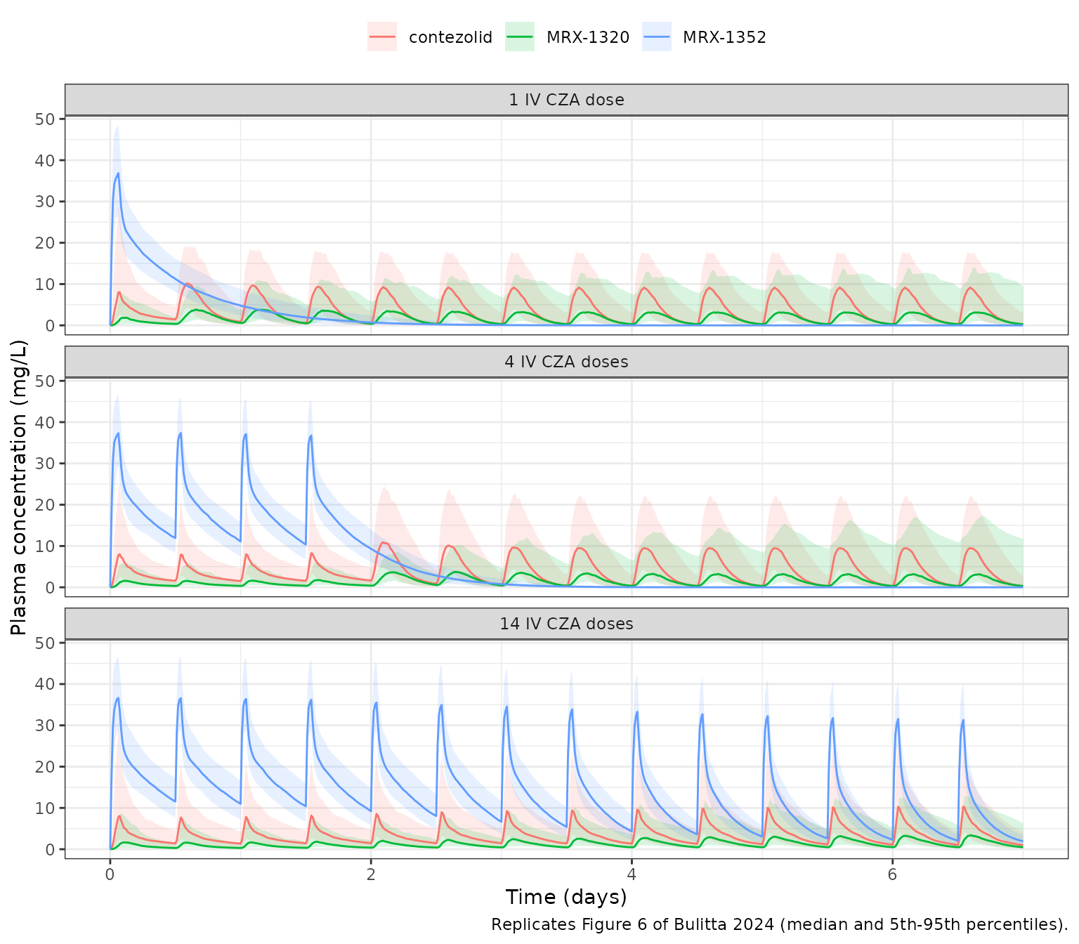
PKNCA of the Monte Carlo cohort
Daily AUCs (days 1, 3 and 7) are computed with PKNCA separately for each analyte and compared against the Table 3 medians.
nca_one <- function(sim, conc_col, analyte) {
  conc <- sim |>
    dplyr::select(id, time, treatment, Cc = dplyr::all_of(conc_col)) |>
    dplyr::filter(!is.na(Cc))
  dose <- mc_events |>
    dplyr::filter(evid == 1) |>
    dplyr::select(id, time, amt, treatment)
  res <- PKNCA::pk.nca(PKNCA::PKNCAdata(
    PKNCA::PKNCAconc(conc, Cc ~ time | treatment + id),
    PKNCA::PKNCAdose(dose, amt ~ time | treatment + id),
    intervals = data.frame(
      start = c(0, 48, 144), end = c(24, 72, 168), auclast = TRUE
    )
  ))
  as.data.frame(res) |>
    dplyr::mutate(analyte = analyte, day = end / 24)
}

mc_nca <- dplyr::bind_rows(
  nca_one(mc_sim, "Cc", "contezolid"),
  nca_one(mc_sim, "Cc_mrx1352", "MRX-1352"),
  nca_one(mc_sim, "Cc_mrx1320", "MRX-1320")
)
#> Warning in assert_conc(conc, any_missing_conc = any_missing_conc): Negative
#> concentrations found
#> Warning in assert_conc(conc, any_missing_conc = any_missing_conc): Negative
#> concentrations found
#> Warning in log(conc.2/conc.1): NaNs produced
#> Warning in assert_conc(conc, any_missing_conc = any_missing_conc): Negative
#> concentrations found
#> Warning in log(conc.2/conc.1): NaNs produced
#> Warning in assert_conc(conc, any_missing_conc = any_missing_conc): Negative
#> concentrations found
#> Warning in log(conc.2/conc.1): NaNs produced
#> Warning in assert_conc(conc, any_missing_conc = any_missing_conc): Negative
#> concentrations found
#> Warning in log(conc.2/conc.1): NaNs produced
#> Warning in assert_conc(conc, any_missing_conc = any_missing_conc): Negative
#> concentrations found
#> Warning in log(conc.2/conc.1): NaNs produced
#> Warning in assert_conc(conc, any_missing_conc = any_missing_conc): Negative
#> concentrations found
#> Warning in log(conc.2/conc.1): NaNs produced
#> Warning in assert_conc(conc, any_missing_conc = any_missing_conc): Negative
#> concentrations found
#> Warning in log(conc.2/conc.1): NaNs produced
#> Warning in assert_conc(conc, any_missing_conc = any_missing_conc): Negative
#> concentrations found
#> Warning in log(conc.2/conc.1): NaNs produced
#> Warning in assert_conc(conc, any_missing_conc = any_missing_conc): Negative
#> concentrations found
#> Warning in log(conc.2/conc.1): NaNs produced
#> Warning in assert_conc(conc, any_missing_conc = any_missing_conc): Negative
#> concentrations found
#> Warning in log(conc.2/conc.1): NaNs produced
#> Warning in assert_conc(conc, any_missing_conc = any_missing_conc): Negative
#> concentrations found
#> Warning in log(conc.2/conc.1): NaNs produced
#> Warning in assert_conc(conc, any_missing_conc = any_missing_conc): Negative
#> concentrations found
#> Warning in log(conc.2/conc.1): NaNs produced
#> Warning in assert_conc(conc, any_missing_conc = any_missing_conc): Negative
#> concentrations found
#> Warning in log(conc.2/conc.1): NaNs produced
#> Warning in assert_conc(conc, any_missing_conc = any_missing_conc): Negative
#> concentrations found
#> Warning in log(conc.2/conc.1): NaNs produced
#> Warning in assert_conc(conc, any_missing_conc = any_missing_conc): Negative
#> concentrations found
#> Warning in log(conc.2/conc.1): NaNs produced
#> Warning in assert_conc(conc, any_missing_conc = any_missing_conc): Negative
#> concentrations found
#> Warning in log(conc.2/conc.1): NaNs produced
#> Warning in assert_conc(conc, any_missing_conc = any_missing_conc): Negative
#> concentrations found
#> Warning in log(conc.2/conc.1): NaNs produced
#> Warning in assert_conc(conc, any_missing_conc = any_missing_conc): Negative
#> concentrations found
#> Warning in log(conc.2/conc.1): NaNs produced
#> Warning in assert_conc(conc, any_missing_conc = any_missing_conc): Negative
#> concentrations found
#> Warning in log(conc.2/conc.1): NaNs produced
#> Warning in assert_conc(conc, any_missing_conc = any_missing_conc): Negative
#> concentrations found
#> Warning in log(conc.2/conc.1): NaNs produced
#> Warning in assert_conc(conc, any_missing_conc = any_missing_conc): Negative
#> concentrations found
#> Warning in log(conc.2/conc.1): NaNs produced
#> Warning in assert_conc(conc, any_missing_conc = any_missing_conc): Negative
#> concentrations found
#> Warning in log(conc.2/conc.1): NaNs produced
#> Warning in assert_conc(conc, any_missing_conc = any_missing_conc): Negative
#> concentrations found
#> Warning in log(conc.2/conc.1): NaNs produced
#> Warning in assert_conc(conc, any_missing_conc = any_missing_conc): Negative
#> concentrations found
#> Warning in log(conc.2/conc.1): NaNs produced
#> Warning in assert_conc(conc, any_missing_conc = any_missing_conc): Negative
#> concentrations found
#> Warning in log(conc.2/conc.1): NaNs produced
#> Warning in assert_conc(conc, any_missing_conc = any_missing_conc): Negative
#> concentrations found
#> Warning in log(conc.2/conc.1): NaNs produced
#> Warning in assert_conc(conc, any_missing_conc = any_missing_conc): Negative
#> concentrations found
#> Warning in log(conc.2/conc.1): NaNs produced
#> Warning in assert_conc(conc, any_missing_conc = any_missing_conc): Negative
#> concentrations found
#> Warning in log(conc.2/conc.1): NaNs produced
#> Warning in assert_conc(conc, any_missing_conc = any_missing_conc): Negative
#> concentrations found
#> Warning in log(conc.2/conc.1): NaNs produced
#> Warning in assert_conc(conc, any_missing_conc = any_missing_conc): Negative
#> concentrations found
#> Warning in log(conc.2/conc.1): NaNs produced
#> Warning in assert_conc(conc, any_missing_conc = any_missing_conc): Negative
#> concentrations found
#> Warning in log(conc.2/conc.1): NaNs produced
#> Warning in assert_conc(conc, any_missing_conc = any_missing_conc): Negative
#> concentrations found
#> Warning in log(conc.2/conc.1): NaNs produced
#> Warning in assert_conc(conc, any_missing_conc = any_missing_conc): Negative
#> concentrations found
#> Warning in log(conc.2/conc.1): NaNs produced
#> Warning in assert_conc(conc, any_missing_conc = any_missing_conc): Negative
#> concentrations found
#> Warning in log(conc.2/conc.1): NaNs produced
#> Warning in assert_conc(conc, any_missing_conc = any_missing_conc): Negative
#> concentrations found
#> Warning in log(conc.2/conc.1): NaNs produced
#> Warning in assert_conc(conc, any_missing_conc = any_missing_conc): Negative
#> concentrations found
#> Warning in log(conc.2/conc.1): NaNs produced
#> Warning in assert_conc(conc, any_missing_conc = any_missing_conc): Negative
#> concentrations found
#> Warning in log(conc.2/conc.1): NaNs produced
#> Warning in assert_conc(conc, any_missing_conc = any_missing_conc): Negative
#> concentrations found
#> Warning in log(conc.2/conc.1): NaNs produced
#> Warning in assert_conc(conc, any_missing_conc = any_missing_conc): Negative
#> concentrations found
#> Warning in log(conc.2/conc.1): NaNs produced
#> Warning in assert_conc(conc, any_missing_conc = any_missing_conc): Negative
#> concentrations found
#> Warning in log(conc.2/conc.1): NaNs produced
#> Warning in assert_conc(conc, any_missing_conc = any_missing_conc): Negative
#> concentrations found
#> Warning in log(conc.2/conc.1): NaNs produced
#> Warning in assert_conc(conc, any_missing_conc = any_missing_conc): Negative
#> concentrations found
#> Warning in log(conc.2/conc.1): NaNs produced
#> Warning in assert_conc(conc, any_missing_conc = any_missing_conc): Negative
#> concentrations found
#> Warning in log(conc.2/conc.1): NaNs produced
#> Warning in assert_conc(conc, any_missing_conc = any_missing_conc): Negative
#> concentrations found
#> Warning in log(conc.2/conc.1): NaNs produced
#> Warning in assert_conc(conc, any_missing_conc = any_missing_conc): Negative
#> concentrations found
#> Warning in log(conc.2/conc.1): NaNs produced
#> Warning in assert_conc(conc, any_missing_conc = any_missing_conc): Negative
#> concentrations found
#> Warning in log(conc.2/conc.1): NaNs produced
#> Warning in assert_conc(conc, any_missing_conc = any_missing_conc): Negative
#> concentrations found
#> Warning in log(conc.2/conc.1): NaNs produced
#> Warning in assert_conc(conc, any_missing_conc = any_missing_conc): Negative
#> concentrations found
#> Warning in log(conc.2/conc.1): NaNs produced
#> Warning in assert_conc(conc, any_missing_conc = any_missing_conc): Negative
#> concentrations found
#> Warning in log(conc.2/conc.1): NaNs produced
#> Warning in assert_conc(conc, any_missing_conc = any_missing_conc): Negative
#> concentrations found
#> Warning in log(conc.2/conc.1): NaNs produced
#> Warning in assert_conc(conc, any_missing_conc = any_missing_conc): Negative
#> concentrations found
#> Warning in log(conc.2/conc.1): NaNs produced
#> Warning in assert_conc(conc, any_missing_conc = any_missing_conc): Negative
#> concentrations found
#> Warning in log(conc.2/conc.1): NaNs produced
#> Warning in assert_conc(conc, any_missing_conc = any_missing_conc): Negative
#> concentrations found
#> Warning in log(conc.2/conc.1): NaNs produced
#> Warning in assert_conc(conc, any_missing_conc = any_missing_conc): Negative
#> concentrations found
#> Warning in log(conc.2/conc.1): NaNs produced
#> Warning in assert_conc(conc, any_missing_conc = any_missing_conc): Negative
#> concentrations found
#> Warning in log(conc.2/conc.1): NaNs produced
#> Warning in assert_conc(conc, any_missing_conc = any_missing_conc): Negative
#> concentrations found
#> Warning in log(conc.2/conc.1): NaNs produced
#> Warning in assert_conc(conc, any_missing_conc = any_missing_conc): Negative
#> concentrations found
#> Warning in log(conc.2/conc.1): NaNs produced
#> Warning in assert_conc(conc, any_missing_conc = any_missing_conc): Negative
#> concentrations found
#> Warning in log(conc.2/conc.1): NaNs produced
#> Warning in assert_conc(conc, any_missing_conc = any_missing_conc): Negative
#> concentrations found
#> Warning in log(conc.2/conc.1): NaNs produced
#> Warning in assert_conc(conc, any_missing_conc = any_missing_conc): Negative
#> concentrations found
#> Warning in log(conc.2/conc.1): NaNs produced
#> Warning in assert_conc(conc, any_missing_conc = any_missing_conc): Negative
#> concentrations found
#> Warning in log(conc.2/conc.1): NaNs produced
#> Warning in assert_conc(conc, any_missing_conc = any_missing_conc): Negative
#> concentrations found
#> Warning in log(conc.2/conc.1): NaNs produced
#> Warning in assert_conc(conc, any_missing_conc = any_missing_conc): Negative
#> concentrations found
#> Warning in log(conc.2/conc.1): NaNs produced
#> Warning in assert_conc(conc, any_missing_conc = any_missing_conc): Negative
#> concentrations found
#> Warning in log(conc.2/conc.1): NaNs produced
#> Warning in assert_conc(conc, any_missing_conc = any_missing_conc): Negative
#> concentrations found
#> Warning in log(conc.2/conc.1): NaNs produced
#> Warning in assert_conc(conc, any_missing_conc = any_missing_conc): Negative
#> concentrations found
#> Warning in log(conc.2/conc.1): NaNs produced
#> Warning in assert_conc(conc, any_missing_conc = any_missing_conc): Negative
#> concentrations found
#> Warning in log(conc.2/conc.1): NaNs produced
#> Warning in assert_conc(conc, any_missing_conc = any_missing_conc): Negative
#> concentrations found
#> Warning in log(conc.2/conc.1): NaNs produced
#> Warning in assert_conc(conc, any_missing_conc = any_missing_conc): Negative
#> concentrations found
#> Warning in log(conc.2/conc.1): NaNs produced
#> Warning in assert_conc(conc, any_missing_conc = any_missing_conc): Negative
#> concentrations found
#> Warning in log(conc.2/conc.1): NaNs produced
#> Warning in assert_conc(conc, any_missing_conc = any_missing_conc): Negative
#> concentrations found
#> Warning in log(conc.2/conc.1): NaNs produced
#> Warning in assert_conc(conc, any_missing_conc = any_missing_conc): Negative
#> concentrations found
#> Warning in log(conc.2/conc.1): NaNs produced
#> Warning in assert_conc(conc, any_missing_conc = any_missing_conc): Negative
#> concentrations found
#> Warning in log(conc.2/conc.1): NaNs produced
#> Warning in assert_conc(conc, any_missing_conc = any_missing_conc): Negative
#> concentrations found
#> Warning in log(conc.2/conc.1): NaNs produced
#> Warning in assert_conc(conc, any_missing_conc = any_missing_conc): Negative
#> concentrations found
#> Warning in log(conc.2/conc.1): NaNs produced
#> Warning in assert_conc(conc, any_missing_conc = any_missing_conc): Negative
#> concentrations found
#> Warning in log(conc.2/conc.1): NaNs produced
#> Warning in assert_conc(conc, any_missing_conc = any_missing_conc): Negative
#> concentrations found
#> Warning in log(conc.2/conc.1): NaNs produced
#> Warning in assert_conc(conc, any_missing_conc = any_missing_conc): Negative
#> concentrations found
#> Warning in log(conc.2/conc.1): NaNs produced
#> Warning in assert_conc(conc, any_missing_conc = any_missing_conc): Negative
#> concentrations found
#> Warning in log(conc.2/conc.1): NaNs produced
#> Warning in assert_conc(conc, any_missing_conc = any_missing_conc): Negative
#> concentrations found
#> Warning in log(conc.2/conc.1): NaNs produced
#> Warning in assert_conc(conc, any_missing_conc = any_missing_conc): Negative
#> concentrations found
#> Warning in log(conc.2/conc.1): NaNs produced
#> Warning in assert_conc(conc, any_missing_conc = any_missing_conc): Negative
#> concentrations found
#> Warning in log(conc.2/conc.1): NaNs produced
#> Warning in assert_conc(conc, any_missing_conc = any_missing_conc): Negative
#> concentrations found
#> Warning in log(conc.2/conc.1): NaNs produced
#> Warning in assert_conc(conc, any_missing_conc = any_missing_conc): Negative
#> concentrations found
#> Warning in log(conc.2/conc.1): NaNs produced
#> Warning in assert_conc(conc, any_missing_conc = any_missing_conc): Negative
#> concentrations found
#> Warning in log(conc.2/conc.1): NaNs produced
#> Warning in assert_conc(conc, any_missing_conc = any_missing_conc): Negative
#> concentrations found
#> Warning in log(conc.2/conc.1): NaNs produced
#> Warning in assert_conc(conc, any_missing_conc = any_missing_conc): Negative
#> concentrations found
#> Warning in log(conc.2/conc.1): NaNs produced
#> Warning in assert_conc(conc, any_missing_conc = any_missing_conc): Negative
#> concentrations found
#> Warning in log(conc.2/conc.1): NaNs produced
#> Warning in assert_conc(conc, any_missing_conc = any_missing_conc): Negative
#> concentrations found
#> Warning in log(conc.2/conc.1): NaNs produced
#> Warning in assert_conc(conc, any_missing_conc = any_missing_conc): Negative
#> concentrations found
#> Warning in log(conc.2/conc.1): NaNs produced
#> Warning in assert_conc(conc, any_missing_conc = any_missing_conc): Negative
#> concentrations found
#> Warning in log(conc.2/conc.1): NaNs produced
#> Warning in assert_conc(conc, any_missing_conc = any_missing_conc): Negative
#> concentrations found
#> Warning in log(conc.2/conc.1): NaNs produced
#> Warning in assert_conc(conc, any_missing_conc = any_missing_conc): Negative
#> concentrations found
#> Warning in log(conc.2/conc.1): NaNs produced
#> Warning in assert_conc(conc, any_missing_conc = any_missing_conc): Negative
#> concentrations found
#> Warning in log(conc.2/conc.1): NaNs produced
#> Warning in assert_conc(conc, any_missing_conc = any_missing_conc): Negative
#> concentrations found
#> Warning in log(conc.2/conc.1): NaNs produced
#> Warning in assert_conc(conc, any_missing_conc = any_missing_conc): Negative
#> concentrations found
#> Warning in log(conc.2/conc.1): NaNs produced
#> Warning in assert_conc(conc, any_missing_conc = any_missing_conc): Negative
#> concentrations found
#> Warning in log(conc.2/conc.1): NaNs produced

reference_mc <- published_t3 |>
  dplyr::filter(day %in% c(1, 3, 7), published >= 5) |>
  dplyr::rename(treatment = regimen, auclast = published)

cmp_mc <- nlmixr2lib::ncaComparisonTable(
  simulated = mc_nca |> dplyr::semi_join(reference_mc, by = c("treatment", "day", "analyte")),
  reference = reference_mc,
  by = c("treatment", "analyte", "day"),
  units = c(auclast = "mg*h/L"),
  tolerance_pct = 20
)
knitr::kable(
  cmp_mc,
  caption = "Median daily AUC of 200 simulated patients per regimen vs Bulitta 2024 Table 3 medians. * differs by >20%."
)| NCA parameter | treatment | analyte | day | Reference | Simulated | % diff |
|---|---|---|---|---|---|---|
| AUClast (mg*h/L) | 1 IV CZA dose | contezolid | 1 | 103 | 99.6 | -3.3% |
| AUClast (mg*h/L) | 1 IV CZA dose | contezolid | 3 | 95.9 | 96.2 | +0.3% |
| AUClast (mg*h/L) | 1 IV CZA dose | contezolid | 7 | 94.1 | 94.7 | +0.7% |
| AUClast (mg*h/L) | 1 IV CZA dose | MRX-1352 | 1 | 334 | 321 | -4.0% |
| AUClast (mg*h/L) | 1 IV CZA dose | MRX-1352 | 3 | 7.36 | 6.76 | -8.2% |
| AUClast (mg*h/L) | 1 IV CZA dose | MRX-1320 | 1 | 36.9 | 37.4 | +1.5% |
| AUClast (mg*h/L) | 1 IV CZA dose | MRX-1320 | 3 | 42.7 | 46 | +7.8% |
| AUClast (mg*h/L) | 1 IV CZA dose | MRX-1320 | 7 | 40.3 | 39.7 | -1.5% |
| AUClast (mg*h/L) | 4 IV CZA doses | contezolid | 1 | 76.3 | 83 | +8.8% |
| AUClast (mg*h/L) | 4 IV CZA doses | contezolid | 3 | 106 | 116 | +9.0% |
| AUClast (mg*h/L) | 4 IV CZA doses | contezolid | 7 | 89.6 | 98.9 | +10.3% |
| AUClast (mg*h/L) | 4 IV CZA doses | MRX-1352 | 1 | 461 | 462 | +0.2% |
| AUClast (mg*h/L) | 4 IV CZA doses | MRX-1352 | 3 | 93.2 | 84.7 | -9.2% |
| AUClast (mg*h/L) | 4 IV CZA doses | MRX-1320 | 1 | 19.3 | 20.4 | +5.7% |
| AUClast (mg*h/L) | 4 IV CZA doses | MRX-1320 | 3 | 50.6 | 48.3 | -4.5% |
| AUClast (mg*h/L) | 4 IV CZA doses | MRX-1320 | 7 | 39.4 | 39.3 | -0.2% |
| AUClast (mg*h/L) | 14 IV CZA doses | contezolid | 1 | 76.8 | 73.3 | -4.5% |
| AUClast (mg*h/L) | 14 IV CZA doses | contezolid | 3 | 84.8 | 84.7 | -0.1% |
| AUClast (mg*h/L) | 14 IV CZA doses | contezolid | 7 | 98.4 | 98.7 | +0.3% |
| AUClast (mg*h/L) | 14 IV CZA doses | MRX-1352 | 1 | 467 | 453 | -3.1% |
| AUClast (mg*h/L) | 14 IV CZA doses | MRX-1352 | 3 | 384 | 369 | -4.0% |
| AUClast (mg*h/L) | 14 IV CZA doses | MRX-1352 | 7 | 218 | 215 | -1.5% |
| AUClast (mg*h/L) | 14 IV CZA doses | MRX-1320 | 1 | 19.6 | 20.9 | +6.5% |
| AUClast (mg*h/L) | 14 IV CZA doses | MRX-1320 | 3 | 27.9 | 26.4 | -5.3% |
| AUClast (mg*h/L) | 14 IV CZA doses | MRX-1320 | 7 | 42.3 | 43 | +1.7% |
All simulated medians fall within about 10% of the published medians, with no row beyond the 20% flag; the largest differences are the contezolid AUCs of the 4-dose regimen, which the simulation places about 9-10% above Table 3.
mc_med <- mc_nca |>
  dplyr::filter(PPTESTCD == "auclast") |>
  dplyr::group_by(treatment, analyte, day) |>
  dplyr::summarise(sim = median(PPORRES), .groups = "drop") |>
  dplyr::inner_join(
    reference_mc |> dplyr::rename(published = auclast),
    by = c("treatment", "analyte", "day")
  ) |>
  dplyr::mutate(pct_diff = 100 * (sim - published) / published)
stopifnot(nrow(mc_med) == nrow(reference_mc))
# Centre and envelope of the cohort medians, not per-cell extremes (the
# cohort differs across rxode2 builds and thread counts).
stopifnot(
  abs(median(mc_med$pct_diff)) < 10,
  quantile(abs(mc_med$pct_diff), 0.9) < 25
)
Assumptions and deviations
- Superseded abstract. The IDWeek 2021 abstract is the preliminary report of this analysis. Its apparent contezolid clearances (13.1 and 14.5 L/h) and steady-state volume (20.5 L) differ from the final paper (16.0 and 17.7 L/h apparent; 17.1 L true Vss). The model uses only the 2024 values.
-
Between-subject variability scale. Table 2 reports
BSV as the ‘apparent coefficient of variation of a normal distribution
on natural logarithmic scale’, i.e. the SD of the log-scale random
effect, so each variance is BSV^2 (the S-ADAPT convention of this group,
as in
Bulitta_2019_pefloxacin). For the large terms the alternativelog(1 + CV^2)reading would differ materially (CLd of contezolid: 1.877 vs 1.066). - Allometric scaling of MRX-1320 and of the two Vmax terms. The Methods state that all clearances (exponent 0.75) and volumes (1.0) were scaled to 70 kg. Table 2 footnote a, which also carries the division-by-F note, marks the contezolid, CZA Vmax and MRX-1352 clearances and volumes but not the MRX-1320 rows. The maintainers followed the Methods statement and scaled every clearance, both Michaelis-Menten maximum rates (as clearance-like capacities) and every volume; AM50, EC50 and Km are not scaled. At the 70 kg reference weight the choice has no effect.
-
Time after first dose. The time-dependent MRX-1352
clearance uses time past the first dose; the model uses solver time
t, so a data set must start at the first dose. -
Occasions for the between-occasion variability of
F. The paper does not define the occasions. Two occasion slots
are provided (the two crossover periods of the single-dose food-effect
part of MRX-I-02);
OCCvalues other than 1 or 2 switch the BOV off. The simulations above useOCC = 1. - Dose-level bands for the relative bioavailability. Table 2 gives F_rel only at 400, 800 and 1200 mg. The model applies the 400 mg row below 600 mg, the 800 mg row from 600 to 1000 mg and the 1200 mg row above 1000 mg.
-
Residual error form. The paper states a combined
additive and proportional residual error without giving the combination
rule; the nlmixr2 default (variances added) is used. Contezolid and
MRX-1320 have separate terms after IV CZA
(
STUDY_MRX4002 = 1) and after oral contezolid. - Numerical guard. The MRX-1352 concentration in the Hill term is floored at zero, because solver round-off after washout can give tiny negative values and a negative number raised to the non-integer Hill coefficient is not defined. This does not change any positive-concentration prediction.
- Monte Carlo design. 200 patients per regimen instead of 1,000, the 56-IV-dose regimen and days 14 and 28 are not simulated, and body weight is truncated to 40-120 kg. The paper’s Monte Carlo was run in Berkeley Madonna; its treatment of the fixed BSV terms and of the BOV is not described, and all model random effects are included here.
- Supplement. The supplement (additional modelling details and diagnostic plots, Figures S1-S3) was not available to the maintainers. The main text, Table 2, equations 1-7 and Figure 2 fully specify the structural model; the close typical-value reproduction of Table 3 indicates that nothing structural was lost.