Aripiprazole once monthly (Wang 2022)
Source:vignettes/articles/Wang_2022_aripiprazole.Rmd
Wang_2022_aripiprazole.RmdModel and source
Wang 2022 contributes two models to nlmixr2lib:
-
modellib("Wang_2022_aripiprazole")– the population PK model for oral aripiprazole and for aripiprazole once monthly (AOM), the intramuscular extended-release injectable suspension. -
modellib("Wang_2022_aripiprazole_relapse")– the exposure-response time-to-event model relating the model-predicted aripiprazole minimum concentration to the time to exacerbation of psychotic symptoms / impending relapse.
The two are independent fits sharing one data programme: the popPK
model produces the individual CMIN_ARI values that the
exposure-response model consumes, but the survival regression was run in
SAS on those predictions rather than estimated jointly. They are
therefore packaged as two model files and validated in this one
vignette.
- Citation: Wang X, Raoufinia A, Bihorel S, Passarell J, Mallikaarjun S, Phillips L. Population Pharmacokinetic Modeling and Exposure-Response Analysis for Aripiprazole Once Monthly in Subjects With Schizophrenia. Clin Pharmacol Drug Dev. 2022;11(2):150-164. doi:10.1002/cpdd.1022.
- Article: https://doi.org/10.1002/cpdd.1022
Population
The population PK model was built from 6153 aripiprazole plasma concentrations in 663 subjects pooled across five studies: four phase 1 studies with serial PK sampling (31-98-206, 31-98-207, CN138020 and 31-05-244) and one phase 3 study with sparse PK sampling (31-07-246). Fifty-two subjects were healthy volunteers who received oral aripiprazole only; the remaining 611 had schizophrenia or schizoaffective disorder. Body mass index ranged from 15 to 61 kg/m^2. CYP2D6 phenotype was extensive in 621 subjects and poor in 42; 13 extensive metabolizers took a concomitant CYP2D6 inhibitor and 25 a concomitant CYP3A4 inhibitor. All AOM doses were given in the gluteus maximus except in study CN138020 (13 subjects, non-dominant arm or midlateral thigh).
A sixth study, phase 3 study 31-07-247, was reserved for external validation. The final model met the pre-specified acceptance criteria for the 400/300 mg AOM arm (median %PPE -6.8%, median |%PPE| 29.2%) but not for the 50/25 mg arm (median |%PPE| 41.3%, 75th percentile 74.6%), so the model must not be extrapolated below 300 mg AOM. Every simulation in this vignette stays at or above 300 mg AOM, or on the 10-30 mg/day oral range the paper used to define its therapeutic window.
The exposure-response analysis set is a different, smaller population: 615 subjects with schizophrenia from the randomised stages of studies 31-07-246 and 31-07-247 (120 on oral aripiprazole, 495 on 400/300 mg AOM, plus the placebo arms), contributing 85 impending-relapse events and 530 censored subjects. The 121 subjects on 50/25 mg AOM were excluded for the reason above.
The same information is available programmatically via each model’s
population metadata
(readModelDb("Wang_2022_aripiprazole")()$population).
Source trace
Every ini() entry carries an in-file comment naming its
source location. The table below collects them.
Population PK model (Wang_2022_aripiprazole)
| Equation / parameter | Value | Source location |
|---|---|---|
lr1 (R1, zero-order oral input rate) |
9.33 mg/h (fixed) | Table 1, row “R1: infusion rate of oral dose into depot compartment (mg/h)” |
lka_oral |
0.540 /h (fixed) | Table 1, row “Ka: oral first-order absorption rate (1/h)” |
lka_im |
0.000904 /h (%RSE 5.3) | Table 1, row “IM Ka: AOM first-order absorption rate (1/h)” |
e_bmi_ka_im |
-0.975 (%RSE 11.5) | Table 1, row “IM Ka: power for (BMI/28)” |
e_sexf_ka_im |
0.346 (%RSE 28.9) | Table 1, row “IM Ka: proportional shift for men” |
lfdepot_im (F2) |
1.48 (%RSE 4.9) | Table 1, row “F2: relative bioavailability for AOM” |
lcl_em |
3.71 L/h (%RSE 4.0) | Table 1, row “CL/F: clearance for EM (L/h)” |
lcl_pm |
1.88 L/h (%RSE 6.9) | Table 1, row “CL/F: clearance for PM (L/h)” |
e_cyp2d6_inh_cl |
-0.511 (fixed) | Table 1, row “CL/F: proportional change in CL/F for CYP2D6 inhibitor” |
e_cyp3a4_inh_cl |
-0.237 (fixed) | Table 1, row “CL/F: proportional change in CL/F for CYP3A4 inhibitor” |
lvc |
93.4 L (%RSE 8.8) | Table 1, row “Vc/F: central volume (L)” |
lq |
0.591 L/h (fixed) | Table 1, row “Q1/F: intercompartmental CL/F (L/h)” |
lvp |
118 L (fixed) | Table 1, row “Vp1/F: peripheral volume (L)” |
lq2 |
28.8 L/h (fixed) | Table 1, row “Q2/F: second intercompartmental CL/F (L/h)” |
lvp2 |
134 L (fixed) | Table 1, row “Vp2/F: second peripheral volume (L)” |
etalcl |
38.34 %CV (%RSE 6.9) | Table 1, IIV column, CL/F row |
etalvc |
124.50 %CV (%RSE 15.2) | Table 1, IIV column, Vc/F row |
etalka_oral |
65.88 %CV (fixed) | Table 1, IIV column, oral Ka row |
etalka_im |
55.59 %CV (%RSE 8.2) | Table 1, IIV column, IM Ka row |
propSdPhase1 |
24.23 %CV (%RSE 8.4) | Table 1, row “Phase 1 RV (%CV)” |
propSdPhase3 |
28.11 %CV (%RSE 4.7) | Table 1, row “Phase 3 RV (%CV)” |
| AOM Ka covariate equation | 0.000904 * (BMI/28)^-0.975 * (1 + 0.346 * Male) |
Table 1 footnote, “Related equations” |
| CL/F covariate equation | (3.71 * EM + 1.88 * PM) * (1 - 0.511 * CYP2D6) * (1 - 0.237 * CYP3A4) |
Table 1 footnote, “Related equations” |
| Three-compartment linear disposition | n/a | Results, “Base Model Development” and “Final PopPK Model” |
| Sigmoid (zero-order then first-order) oral absorption; first-order AOM absorption | n/a | Results, “Base Model Development”; Table 1 footnote |
| Which parameters were estimated vs carried over fixed | n/a | Results, “Base Model Development” and “Final PopPK Model” |
Exposure-response model
(Wang_2022_aripiprazole_relapse)
| Equation / parameter | Value | Source location |
|---|---|---|
lhaz_base |
-6.256 (= -1 x 6.256; SE 0.1474, 95% CI 5.97-6.55) | Table 2, row “Intercept” |
e_cmin_haz |
-1.484 (= -1 x 1.484; SE 0.2177, 95% CI 1.06-1.91) | Table 2, row “Predicted aripiprazole (Cmin >= 95 ng/mL) proximate to the event” |
Hazard ratio exp(-e_cmin_haz) = 4.41 (95% CI
2.89-6.75) |
4.41 | Table 2, row “Calculated hazard ratio of expected survival time” |
| 95 ng/mL threshold | 95 ng/mL | Results, “Exposure-Response Analysis of Time to Relapse” |
| Exponential (constant-hazard) functional form | n/a | Results, “Exposure-Response Analysis of Time to Relapse” |
| Time unit = days | n/a | Figures 5 and 6 x-axis label, “Time to Relapse (days)” |
The only non-transcription step in either file is the survival-model
parameterisation. Wang 2022 Table 2 reports an accelerated-failure-time
exponential regression on log survival time (SAS
PROC LIFEREG),
log(T) = 6.256 + 1.484 * I(Cmin >= 95). For the
exponential distribution the constant hazard is the reciprocal of the
expected survival time, so the log-hazard parameters are the negatives
of the printed ones. The sign is confirmed by the paper’s own derived
quantity: exp(1.484) = 4.41 must be a hazard
reduction for subjects at or above the threshold, which is
exactly what exp(-e_cmin_haz) gives below.
Virtual cohort
Original observed data are not publicly available. The cohorts below use covariate distributions that approximate the published trial demographics: 60% men (Wang 2022 Methods, “Population PK Model Simulations”, which specifies the same split for the paper’s own 10 000-subject virtual population) and a CYP2D6 poor-metabolizer prevalence of 42/663 = 6.3% matching the model development set.
BMI is drawn log-normally with a median of 28 kg/m^2 – the reference value the paper’s own AOM Ka equation is centred on – and a geometric CV of 22%. The paper states only that the virtual BMI values were “log-normally distributed on the basis of sex to be similar to the phase 3 population” and reports the observed range (15-61 kg/m^2); the per-sex distribution parameters are in the supplement, which was not available when this model was built. See Assumptions and deviations.
# `set.seed()` seeds R's RNG only. rxode2's own simulation RNG is partitioned
# per solver thread, so the eta draws below differ between a 2-core CI runner
# and a 16-thread workstation. Every assertion in this vignette is therefore
# either deterministic (typical-value solve, closed-form identity) or written
# on a robust central statistic, never on a cohort extreme.
set.seed(20220211)

nPerArm <- 200L

makeSubjects <- function(n, id_offset = 0L, pmFraction = 42 / 663) {
  tibble::tibble(
    id        = id_offset + seq_len(n),
    SEXF      = as.numeric(seq_len(n) > round(0.60 * n)),   # 60% men
    BMI       = round(stats::rlnorm(n, meanlog = log(28), sdlog = 0.22), 2),
    CYP2D6_PM = as.numeric(seq_len(n) <= round(pmFraction * n)),
    CONMED_CYP2D6_INH = 0,
    CONMED_CYP3A4_INH = 0,
    STUDY_ARI_PHASE3  = 1
  )
}

# One arm = subjects x (dose records + observation grid).
# Oral doses use rate = -1 so rxode2 applies the modelled zero-order input
# rate R1 = 9.33 mg/h; AOM doses are ordinary bolus records into `depot2`.
makeArm <- function(subj, cohort, amt, cmt, ii, addl, obsTimes) {
  # Resolve the dose rate from the ARGUMENT before mutate() shadows `cmt` with
  # the newly created (length-n) column of the same name.
  doseRate <- if (identical(cmt, "depot")) -1 else 0
  doses <- subj |>
    dplyr::mutate(
      time = 0, evid = 1L, amt = amt, cmt = cmt,
      rate = doseRate,
      ii = ii, addl = addl
    )
  obs <- subj |>
    tidyr::expand_grid(time = obsTimes) |>
    dplyr::mutate(evid = 0L, amt = 0, cmt = "central", rate = 0, ii = 0, addl = 0L)
  dplyr::bind_rows(doses, obs) |>
    dplyr::mutate(cohort = cohort) |>
    dplyr::arrange(id, time, dplyr::desc(evid))
}

tauAom  <- 672   # 28 days, in hours
tauOral <- 24

# AOM: 31 doses (dose 31 at 20160 h); observe the first interval densely for
# the concentration-time profile and the last interval for steady-state NCA.
obsAom  <- sort(unique(c(seq(0, tauAom, by = 6),
                         seq(30 * tauAom, 31 * tauAom, by = 12))))
# Oral: 91 doses (dose 91 at 2160 h) -- about 12 terminal half-lives.
obsOral <- sort(unique(c(0, seq(90 * tauOral, 91 * tauOral, by = 0.5))))

events <- dplyr::bind_rows(
  makeArm(makeSubjects(nPerArm,   0L), "AOM 400 mg q28d", 400, "depot2", tauAom,  30L, obsAom),
  makeArm(makeSubjects(nPerArm, 200L), "Oral 10 mg QD",    10, "depot",  tauOral, 90L, obsOral),
  makeArm(makeSubjects(nPerArm, 400L), "Oral 30 mg QD",    30, "depot",  tauOral, 90L, obsOral)
)

stopifnot(
  !anyDuplicated(events[events$evid == 0L, c("id", "time")]),
  nPerArm <= 200L
)
Simulation
mod <- readModelDb("Wang_2022_aripiprazole")

sim <- rxode2::rxSolve(mod, events = events, keep = c("cohort", "SEXF", "CYP2D6_PM", "BMI"))
A typical-value (zeroRe) solve supplies the
deterministic checks. Because the paper reports the AOM absorption
half-life, the therapeutic-window bounds and the CYP2D6-poor-metabolizer
dose recommendation as typical-subject quantities, these are the
sharpest gates available.
modTypical <- rxode2::zeroRe(mod)
#> Warning: No sigma parameters in the model

typicalScenario <- function(label, amt, cmt, ii, addl, obsTimes,
                            SEXF = 0, BMI = 28, CYP2D6_PM = 0,
                            CONMED_CYP2D6_INH = 0, CONMED_CYP3A4_INH = 0) {
  subj <- tibble::tibble(
    id = 1L, SEXF = SEXF, BMI = BMI, CYP2D6_PM = CYP2D6_PM,
    CONMED_CYP2D6_INH = CONMED_CYP2D6_INH,
    CONMED_CYP3A4_INH = CONMED_CYP3A4_INH, STUDY_ARI_PHASE3 = 1
  )
  ev <- makeArm(subj, label, amt, cmt, ii, addl, obsTimes)
  rxode2::rxSolve(modTypical, events = ev, omega = NA, keep = "cohort") |>
    as.data.frame()
}

typ <- dplyr::bind_rows(
  typicalScenario("Oral 10 mg QD (EM)",   10, "depot",  tauOral, 90L, obsOral),
  typicalScenario("Oral 30 mg QD (EM)",   30, "depot",  tauOral, 90L, obsOral),
  typicalScenario("AOM 400 mg q28d (EM, men)",  400, "depot2", tauAom, 30L, obsAom),
  typicalScenario("AOM 400 mg q28d (EM, women)", 400, "depot2", tauAom, 30L, obsAom, SEXF = 1),
  typicalScenario("AOM 300 mg q28d (PM, men)",  300, "depot2", tauAom, 30L, obsAom, CYP2D6_PM = 1),
  typicalScenario("AOM 400 mg q28d (PM, men)",  400, "depot2", tauAom, 30L, obsAom, CYP2D6_PM = 1)
)

ssWindow <- function(df, cohort, start, end) {
  d <- df[df$cohort == cohort & df$time >= start & df$time <= end, ]
  list(
    cmin = min(d$Cc), cmax = max(d$Cc),
    auc  = sum(diff(d$time) * (utils::head(d$Cc, -1) + utils::tail(d$Cc, -1)) / 2) / 1000
  )
}
Structural checks against the paper’s own reported quantities
AOM absorption half-life (Results, “Final PopPK Model”)
“For a typical subject with a BMI of 28 [kg/m^2], the estimated AOM absorption half-life was approximately 32 days for women and 24 days for men.”
kaIm <- function(BMI, SEXF) 0.000904 * (BMI / 28)^-0.975 * (1 + 0.346 * (1 - SEXF))
absHalfLifeDays <- c(
  women = log(2) / kaIm(28, 1) / 24,
  men   = log(2) / kaIm(28, 0) / 24
)
round(absHalfLifeDays, 2)
#> women   men
#> 31.95 23.74

# Deterministic: no simulation, no random draw. Tight bound is correct here.
stopifnot(
  abs(absHalfLifeDays[["women"]] - 32) < 0.5,
  abs(absHalfLifeDays[["men"]]   - 24) < 0.5
)
Terminal elimination half-life (Results, “Model Simulations”)
“The average terminal elimination half-life was approximately 7.5 days for men and women.”
The terminal half-life is a property of the disposition parameters, so it is read from the slowest eigenvalue of the three-compartment rate matrix rather than from an NCA. An NCA of an AOM profile would return the absorption half-life instead, because AOM elimination is absorption-rate limited (absorption half-life about 28 days versus 7 days for elimination) – the flip-flop the paper describes in its Discussion.
cl <- 3.71; vc <- 93.4; q <- 0.591; vp <- 118; q2 <- 28.8; vp2 <- 134
rateMatrix <- matrix(
  c(-(cl + q + q2) / vc,  q / vp,  q2 / vp2,
    q / vc,              -q / vp,  0,
    q2 / vc,              0,      -q2 / vp2),
  nrow = 3, byrow = TRUE
)
lambdaZ <- max(Re(eigen(rateMatrix)$values))     # least negative eigenvalue
terminalHalfLifeDays <- log(2) / -lambdaZ / 24
round(terminalHalfLifeDays, 2)
#> [1] 7

stopifnot(terminalHalfLifeDays > 6.5, terminalHalfLifeDays < 8.0)
Therapeutic window (Methods, “Definition of Therapeutic Window”)
“The median of the simulated 10-mg oral minimum predicted drug concentration at steady state (Cmin,ss) values (94.0 ng/mL) was used to establish the minimum of the therapeutic window … the 75th percentile of the simulated 30-mg oral maximum predicted drug concentration at steady state (Cmax,ss) values (534 ng/mL) was selected as a conservative upper bound.”
windowLower <- 94.0
windowUpper <- 534

oralSsStart <- 90 * tauOral
oral10 <- ssWindow(typ, "Oral 10 mg QD (EM)", oralSsStart, oralSsStart + tauOral)
oral30 <- ssWindow(typ, "Oral 30 mg QD (EM)", oralSsStart, oralSsStart + tauOral)

tibble::tibble(
  quantity  = c("Oral 10 mg QD typical Cmin,ss", "Oral 30 mg QD typical Cmax,ss"),
  simulated = c(oral10$cmin, oral30$cmax),
  published = c(windowLower, windowUpper),
  statistic = c("median over 10 000 subjects", "75th percentile over 10 000 subjects")
) |>
  dplyr::mutate(`% diff` = 100 * (simulated - published) / published) |>
knitr::kable(digits = 1, caption = "Therapeutic-window bounds (Wang 2022 Methods).")| quantity | simulated | published | statistic | % diff |
|---|---|---|---|---|
| Oral 10 mg QD typical Cmin,ss | 92.1 | 94 | median over 10 000 subjects | -2.0 |
| Oral 30 mg QD typical Cmax,ss | 412.6 | 534 | 75th percentile over 10 000 subjects | -22.7 |
# The typical-value Cmin,ss is the natural estimate of the paper's cohort
# MEDIAN (clearance is log-normal, so the median subject is the typical
# subject). Deterministic, so a 10% bound is appropriate.
stopifnot(abs(oral10$cmin - windowLower) / windowLower < 0.10)
# The 30 mg bound is a 75th PERCENTILE of a cohort with 125 %CV IIV on Vc, so
# the typical-value Cmax,ss must sit below it -- but not absurdly so.
stopifnot(oral30$cmax < windowUpper, oral30$cmax > 0.6 * windowUpper)
CYP2D6 poor metabolizers (Results, “Model Simulations”, Figure 4 panel 2)
“for subjects with a known poor CYP2D6 metabolizer status, median steady-state concentrations after dosing of 300-mg AOM (as recommended) remained centered within the therapeutic window, while concentrations following dosing of 400-mg AOM approached the upper limit of the therapeutic window.”
This is the single tightest cross-check available: reproducing “400
mg AOM in a poor metabolizer approaches 534 ng/mL” requires
lcl_pm, lfdepot_im, lka_im,
lvc and the whole three-compartment disposition to be
simultaneously correct.
aomSsStart <- 30 * tauAom
pm300 <- ssWindow(typ, "AOM 300 mg q28d (PM, men)", aomSsStart, aomSsStart + tauAom)
pm400 <- ssWindow(typ, "AOM 400 mg q28d (PM, men)", aomSsStart, aomSsStart + tauAom)

tibble::tibble(
  scenario = c("300 mg AOM, CYP2D6 PM", "400 mg AOM, CYP2D6 PM"),
  `Cmin,ss (ng/mL)` = c(pm300$cmin, pm400$cmin),
  `Cmax,ss (ng/mL)` = c(pm300$cmax, pm400$cmax)
) |>
  knitr::kable(digits = 1,
caption = "Typical-value steady state in CYP2D6 poor metabolizers; therapeutic window 94.0-534 ng/mL.")| scenario | Cmin,ss (ng/mL) | Cmax,ss (ng/mL) |
|---|---|---|
| 300 mg AOM, CYP2D6 PM | 275.9 | 399.6 |
| 400 mg AOM, CYP2D6 PM | 367.9 | 532.8 |
Replicate published figures
# Replicates Figure 1 of Wang 2022 (left column): mean aripiprazole
# concentration-time profile following the FIRST AOM injection.
sim |>
  dplyr::filter(cohort == "AOM 400 mg q28d", time <= tauAom) |>
  dplyr::group_by(time) |>
  dplyr::summarise(
    Q05 = quantile(Cc, 0.05), Q50 = median(Cc), Q95 = quantile(Cc, 0.95),
    .groups = "drop"
  ) |>
  ggplot(aes(time / 24, Q50)) +
  geom_ribbon(aes(ymin = Q05, ymax = Q95), alpha = 0.25) +
  geom_line() +
  labs(x = "Days since first injection", y = "Aripiprazole (ng/mL)",
       title = "Figure 1 (left column) - first 400 mg AOM injection",
       caption = "Median and 5th-95th percentiles, 200 virtual subjects. Replicates Figure 1 of Wang 2022.")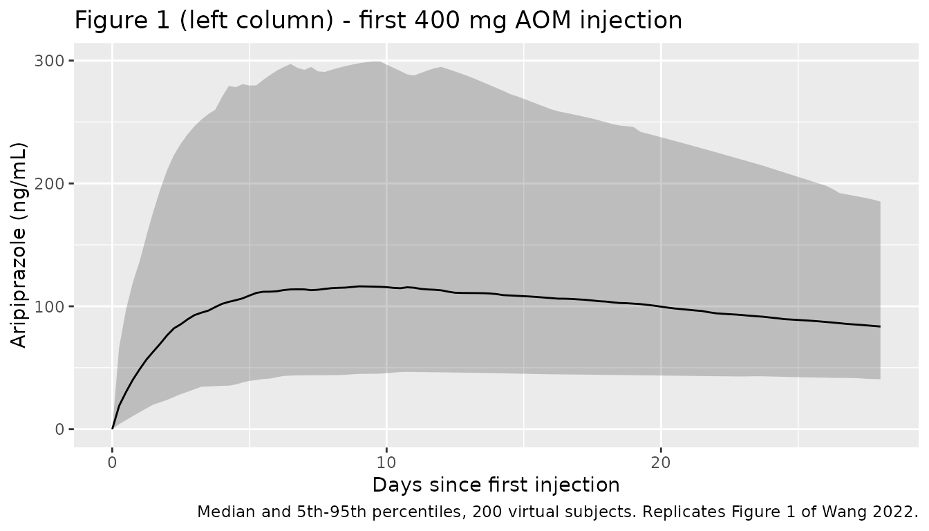
# Replicates Figure 4 panel 2 of Wang 2022: steady-state concentration versus
# days since the previous active dose, for CYP2D6 poor and extensive
# metabolizers, against the therapeutic window.
typ |>
  dplyr::filter(grepl("^AOM", cohort), time >= aomSsStart) |>
  dplyr::mutate(daysSinceDose = (time - aomSsStart) / 24) |>
  ggplot(aes(daysSinceDose, Cc, colour = cohort)) +
  geom_line() +
  geom_hline(yintercept = c(windowLower, windowUpper), linetype = "dashed") +
  labs(x = "Days since previous active dose", y = "Aripiprazole (ng/mL)",
       colour = NULL,
       title = "Figure 4 panel 2 - steady state by CYP2D6 phenotype and dose",
       caption = "Typical-value profiles; dashed lines are the 94.0-534 ng/mL therapeutic window. Replicates Figure 4 panel 2 of Wang 2022.")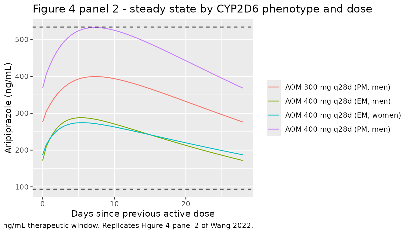
PKNCA validation
simNca <- sim |>
  dplyr::filter(!is.na(Cc)) |>
  dplyr::select(id, time, Cc, cohort)

# Defensive time-zero record (pre-dose extravascular concentration is 0).
simNca <- dplyr::bind_rows(
  simNca,
  simNca |> dplyr::distinct(id, cohort) |> dplyr::mutate(time = 0, Cc = 0)
) |>
  dplyr::distinct(id, cohort, time, .keep_all = TRUE) |>
  dplyr::arrange(id, cohort, time)

concObj <- PKNCA::PKNCAconc(simNca, Cc ~ time | cohort + id,
                            concu = "ng/mL", timeu = "h")

doseDf <- events |>
  dplyr::filter(evid == 1L) |>
  dplyr::select(id, time, amt, cohort)

doseObj <- PKNCA::PKNCAdose(doseDf, amt ~ time | cohort + id, doseu = "mg")

# One steady-state interval per cohort: the last complete dosing interval.
intervals <- data.frame(
  cohort  = c("AOM 400 mg q28d", "Oral 10 mg QD", "Oral 30 mg QD"),
  start   = c(aomSsStart, oralSsStart, oralSsStart),
  end     = c(aomSsStart + tauAom, oralSsStart + tauOral, oralSsStart + tauOral),
  cmax    = TRUE,
  cmin    = TRUE,
  auclast = TRUE,
  cav     = TRUE,
  stringsAsFactors = FALSE
)

ncaRes <- PKNCA::pk.nca(PKNCA::PKNCAdata(concObj, doseObj, intervals = intervals))

ncaWide <- as.data.frame(ncaRes) |>
  dplyr::select(cohort, id, PPTESTCD, PPORRES) |>
  tidyr::pivot_wider(names_from = PPTESTCD, values_from = PPORRES)
Comparison against published NCA
Wang 2022 summarises each of these three regimens with a different statistic, so each row below is summarised the same way the paper summarised it – means for the 400 mg AOM steady-state exposures (Results, “Model Simulations”), the median for the 10 mg oral Cmin,ss and the 75th percentile for the 30 mg oral Cmax,ss (Methods, “Definition of Therapeutic Window”). The statistic used is named in the table caption and repeated per row below.
summariseCohort <- function(df, cohort, fn) {
  d <- df[df$cohort == cohort, ]
  tibble::tibble(
    cohort  = cohort,
    cmax    = fn(d$cmax),
    cmin    = fn(d$cmin),
    auclast = fn(d$auclast)
  )
}

simulatedSummary <- dplyr::bind_rows(
  summariseCohort(ncaWide, "AOM 400 mg q28d", mean),
  summariseCohort(ncaWide, "Oral 10 mg QD",   median),
  summariseCohort(ncaWide, "Oral 30 mg QD",   function(x) stats::quantile(x, 0.75))
)

# Published reference values. AUC0-tau,ss 178.5 mg*h/L = 178 500 ng*h/mL.
# The oral rows report only the one bound the paper published for that
# regimen, so the other cells are NA and are dropped from the comparison.
published <- tibble::tribble(
  ~cohort,            ~cmax, ~cmin, ~auclast,
  "AOM 400 mg q28d",  321.5, 195.9, 178500,
  "Oral 10 mg QD",    NA,     94.0, NA,
  "Oral 30 mg QD",    534,    NA,   NA
)

cmp <- nlmixr2lib::ncaComparisonTable(
  simulated = simulatedSummary |> dplyr::filter(!is.na(cmax)),
  reference = published,
  by        = "cohort",
  units     = c(cmax = "ng/mL", cmin = "ng/mL", auclast = "ng*h/mL"),
  tolerance_pct = 20
)

knitr::kable(
  cmp,
  caption = paste(
    "Simulated versus published NCA. Each cohort is summarised with the",
    "statistic Wang 2022 used for it: mean (AOM 400 mg), median (oral 10 mg),",
    "75th percentile (oral 30 mg). * marks a difference above 20%."
  ),
  align = c("l", "l", "r", "r", "r")
)| NCA parameter | cohort | Reference | Simulated | % diff |
|---|---|---|---|---|
| Cmax (ng/mL) | AOM 400 mg q28d | 322 | 317 | -1.5% |
| Cmax (ng/mL) | Oral 10 mg QD | — | 149 | — |
| Cmax (ng/mL) | Oral 30 mg QD | 534 | 549 | +2.8% |
| Cmin (ng/mL) | AOM 400 mg q28d | 196 | 205 | +4.5% |
| Cmin (ng/mL) | Oral 10 mg QD | 94 | 104 | +10.4% |
| Cmin (ng/mL) | Oral 30 mg QD | — | 401 | — |
| AUClast (ng*h/mL) | AOM 400 mg q28d | 178000 | 180000 | +0.8% |
| AUClast (ng*h/mL) | Oral 10 mg QD | — | 2910 | — |
| AUClast (ng*h/mL) | Oral 30 mg QD | — | 10900 | — |
aomRow <- simulatedSummary[simulatedSummary$cohort == "AOM 400 mg q28d", ]

# Cohort-level checks. These are means over a 200-subject draw with 125 %CV
# IIV on Vc, so they are sized as envelopes on the CENTRE, not on extremes.
stopifnot(
  abs(aomRow$auclast - 178500) / 178500 < 0.30,
  abs(aomRow$cmax    -  321.5) /  321.5 < 0.30,
  abs(aomRow$cmin    -  195.9) /  195.9 < 0.30
)
Exposure-response: time to impending relapse
The exposure-response model is deterministic (no IIV, no residual error), so every check below is an exact reproduction rather than a statistical one.
modEr <- readModelDb("Wang_2022_aripiprazole_relapse")

erEvents <- dplyr::bind_rows(
  tibble::tibble(id = 1L, CMIN_ARI =  40, cohort = "Cmin < 95 ng/mL"),
  tibble::tibble(id = 2L, CMIN_ARI = 200, cohort = "Cmin >= 95 ng/mL")
) |>
  tidyr::expand_grid(time = seq(0, 365, by = 1)) |>
  dplyr::mutate(evid = 0L, amt = 0, cmt = "cumhaz")

simEr <- rxode2::rxSolve(modEr, events = erEvents, keep = c("cohort", "CMIN_ARI")) |>
  as.data.frame()
# Replicates Figure 6 of Wang 2022: model-predicted probability of survival
# (no relapse) versus time, for predicted Cmin below and at/above 95 ng/mL.
ggplot(simEr, aes(time, sur, colour = cohort)) +
  geom_line() +
  ylim(0, 1) +
  labs(x = "Time to relapse (days)", y = "Probability of survival (no relapse)",
       colour = NULL,
       title = "Figure 6 - relapse-free survival by predicted Cmin group",
       caption = "Replicates the model-predicted median (blue dashed) curves of Figure 6 of Wang 2022.")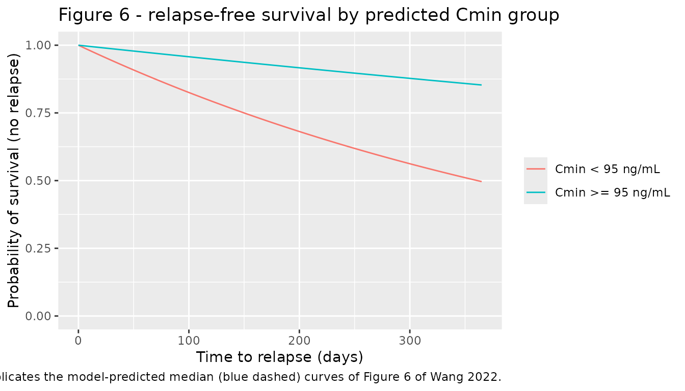
hazards <- simEr |>
  dplyr::group_by(cohort) |>
  dplyr::summarise(hazard = unique(round(hazard, 12)),
                   sur350 = sur[time == 350], .groups = "drop")
hazards
#> # A tibble: 2 × 3
#>   cohort             hazard sur350
#>   <chr>               <dbl>  <dbl>
#> 1 Cmin < 95 ng/mL  0.00192   0.511
#> 2 Cmin >= 95 ng/mL 0.000435  0.859

hazardRatio <- hazards$hazard[hazards$cohort == "Cmin < 95 ng/mL"] /
  hazards$hazard[hazards$cohort == "Cmin >= 95 ng/mL"]

# Table 2 hazard ratio (95% CI 2.89-6.75). Deterministic identity.
stopifnot(abs(hazardRatio - 4.41) < 0.01)

# Figure 6 read-off at about 350 days: the model-predicted (blue dashed)
# survival is about 0.49 in the [0, 95] panel and about 0.86 in the
# (95, 580] panel.
sur350 <- stats::setNames(hazards$sur350, hazards$cohort)
round(sur350, 3)
#>  Cmin < 95 ng/mL Cmin >= 95 ng/mL
#>            0.511            0.859
stopifnot(
  abs(sur350[["Cmin < 95 ng/mL"]]  - 0.49) < 0.05,
  abs(sur350[["Cmin >= 95 ng/mL"]] - 0.86) < 0.05
)

# The exponential model's own closed form, exp(-t / exp(intercept)).
stopifnot(
  abs(sur350[["Cmin < 95 ng/mL"]]  - exp(-350 / exp(6.256)))         < 1e-6,
  abs(sur350[["Cmin >= 95 ng/mL"]] - exp(-350 / exp(6.256 + 1.484))) < 1e-6
)
Assumptions and deviations
Supplement not available. Wang 2022 Tables S1-S4, Figures S1-S3 and Appendices S1-S2 were not available when this model was built. Nothing needed for either model is in them: Table 1 gives every final popPK estimate and both covariate equations, and Table 2 gives both survival parameters. Table S4 holds the base model (before the phase 3 data were added), which the final model supersedes; Tables S2/S3 hold per-study covariate summaries, which is why the
populationmetadata reports the demographic ranges only where the main text states them.Virtual-cohort BMI distribution. Log-normal, median 28 kg/m^2, geometric CV 22%. The paper’s own virtual population used sex-specific log-normal BMI distributions “similar to the phase 3 population” but does not print the parameters (they would be in Table S2). The median is anchored on the 28 kg/m^2 reference value of the paper’s AOM Ka equation; the spread was chosen so the central 95% spans roughly 18-43 kg/m^2. The paper’s observed range, 15-61 kg/m^2, is wider because it includes cohort extremes. This affects only the cohort figures and the cohort NCA row; every structural check in this vignette is run at the reference BMI of 28.
Sex coding is inverted relative to the paper. Wang 2022 writes the AOM Ka covariate on a
Maleindicator; the canonical column isSEXF(1 = female), so the model applies(1 + e_sexf_ka_im * (1 - SEXF)). This is an exact re-expression, verified above by reproducing the paper’s own AOM absorption half-lives (31.95 versus “about 32” days for women; 23.74 versus “about 24” days for men).Survival model reparameterised from AFT to hazard. See the Source trace section. The exponential distribution makes the two parameterisations equivalent; the signs are confirmed by reproducing the paper’s own 4.41 hazard ratio and its Figure 6 survival curves.
IIV variances back-transformed from %CV. Wang 2022 Table 1 reports IIV as percent coefficients of variation. The model file stores
omega^2 = log(CV^2 + 1), so the Vc IIV of 124.50 %CV becomes a variance of 0.936 (omega 0.968) rather than the naive 1.245^2. This is the package convention for log-normally distributed random effects and is documented in the model file.No IIV correlations. Wang 2022 Results, “Covariate Analysis”, states that the off-diagonal covariance elements could not be estimated. The r = 0.901 in the Table 1 footnote is a correlation between the estimates of
lcl_emandlfdepot_im(estimation precision), not an IIV covariance, and is therefore deliberately not encoded as an omega block.The CYP2D6 mixture model is not carried over. For subjects whose CYP2D6 status was unmeasured, Wang 2022 imputed the phenotype with a NONMEM mixture model assuming 90% extensive metabolizers. That is an estimation device for missing covariate data, not part of the final structural model, so
CYP2D6_PMis carried here as an ordinary observed covariate.Do not extrapolate below 300 mg AOM. The model development data set contained no AOM dose below 300 mg, and the paper’s own external validation showed the model does not adequately describe the 50/25 mg arm (median |%PPE| 41.3%, 75th percentile 74.6%). Wang 2022 excluded that arm from its own exposure-response analysis rather than refit.
Terminal half-life is checked analytically, not by NCA. AOM elimination is absorption-rate limited (flip-flop), so an NCA of an AOM profile returns the absorption half-life of roughly 28 days, not the 7.5-day terminal elimination half-life. The check above therefore reads the terminal half-life from the disposition rate matrix. The 7.00 days it returns is the typical-subject value; the paper’s 7.5 days is an average over individual empirical-Bayes estimates that includes the 42 poor metabolizers, whose lower clearance gives them a longer terminal half-life.
Injection site. Every simulation here represents gluteal administration. Injection site was screened as a covariate on AOM Ka and was not retained, but only 13 subjects (study CN138020) received arm or thigh injections, so the model carries no site term and should not be used to predict a site difference. The paper’s Discussion proposes bridging to alternative sites via the 95 ng/mL Cmin threshold rather than via a PK covariate.
Errata
No erratum, corrigendum or author correction to Wang 2022 (doi:10.1002/cpdd.1022) was located.