3D regimen for HCV genotype 1 (Mensing 2017)
Source:vignettes/articles/Mensing_2017_3D_HCV_regimen.Rmd
Mensing_2017_3D_HCV_regimen.RmdModel and source
Mensing et al. (2017) reported population pharmacokinetic models for each of the five components of the 3D + ribavirin regimen for treating chronic hepatitis C virus (HCV) genotype 1 infection:
-
Mensing_2017_paritaprevir- one-compartment with absorption lag time -
Mensing_2017_ombitasvir- one-compartment -
Mensing_2017_dasabuvir- two-compartment -
Mensing_2017_ritonavir- one-compartment (pharmacokinetic enhancer) -
Mensing_2017_ribavirin- two-compartment
All models were fit using NONMEM 7.3 with FOCE-INT, separately per drug. The authors describe the regimen as 3D (three direct-acting antivirals: paritaprevir/r, ombitasvir, dasabuvir) optionally with ribavirin. The analysis pooled data from one phase II study (NCT01911845) and six phase III studies (PEARL-II/III/IV, SAPPHIRE-I/II, TURQUOISE-II), comprising 2,348 subjects for the DAA / ritonavir models and 1,841 subjects for the ribavirin model.
- Article: https://doi.org/10.1111/bcp.13138
Population
mod_ombi <- rxode2::rxode(readModelDb("Mensing_2017_ombitasvir"))
#> ℹ parameter labels from comments will be replaced by 'label()'
cat("Species:           ", mod_ombi$population$species, "\n")
#> Species:            human
cat("N subjects (DAAs): ", mod_ombi$population$n_subjects, "\n")
#> N subjects (DAAs):  2348
cat("Age range:         ", mod_ombi$population$age_range, " (median ",
    mod_ombi$population$age_median, ")\n", sep = "")
#> Age range:         18-71 years (median 54 years)
cat("Weight range:      ", mod_ombi$population$weight_range, " (median ",
    mod_ombi$population$weight_median, ")\n", sep = "")
#> Weight range:      42-129 kg (median 76 kg)
cat("Sex (female):      ", mod_ombi$population$sex_female_pct, "%\n", sep = "")
#> Sex (female):      42%
cat("Disease state:     ", mod_ombi$population$disease_state, "\n")
#> Disease state:      Adults with chronic hepatitis C virus (HCV) genotype 1 infection (HCV RNA > 10,000 IU/mL). 16% had compensated cirrhosis (Child-Pugh A); none had moderate or severe hepatic impairment. 34% were peg-IFN/RBV treatment-experienced.
Adult subjects (18-71 years) with chronic HCV genotype 1 infection (HCV RNA > 10,000 IU/mL) received paritaprevir 150 mg + ritonavir 100 mg + ombitasvir 25 mg coformulated once daily, plus dasabuvir 250 mg twice daily, with or without weight-based ribavirin (1000 mg/day for body weight < 75 kg, 1200 mg/day for body weight >= 75 kg, divided into twice-daily doses), for 12 weeks or 24 weeks (only in patients with compensated cirrhosis). Demographic and clinical baseline characteristics: 42% female, 7% Black, 2% Asian, 6% Hispanic/Latino; 16% with compensated cirrhosis (Child-Pugh A); 34% peg-IFN/RBV treatment-experienced; median creatinine clearance 104 mL/min (range 37.0-281.4); 53% HCV genotype 1a and 47% genotype 1b (source: Mensing 2017 Table 2, DAA pharmacokinetic data column).
Source trace
Per-drug structural parameters and inter-individual variability are reported in Mensing 2017 Table 3 with 95% bootstrap confidence intervals (500 replicates). Significant covariates per drug are listed but their numeric coefficient point estimates are not published; only Figure 2 graphical exposure-ratio forest plots are reported. The implemented models therefore encode only structural typical values (see Assumptions and deviations).
| Drug | Compartments | ka (1/day) | CL/F (L/day) | Vc/F (L) | Q/F (L/day) | Vp/F (L) | Residual error |
|---|---|---|---|---|---|---|---|
| Paritaprevir | 1, with lag | 1.74 (fixed) | 1580 (1450, 1710) | 16.7 (11.8, 22.6) | - | - | additive on log-transformed: sigma^2 = 1.14 (1.09, 1.20) |
| Ombitasvir | 1 | 1.08 (1.01, 1.14) | 453 (441, 467) | 50.1 (44.9, 55.8) | - | - | prop. 0.107 + add. 2.4e-5 |
| Dasabuvir | 2 | 4.61 (3.99, 5.45) | 1150 (1100, 1200) | 110 (93.3, 133) | 182 (111, 295) | 286 (190, 408) | prop. 0.260 + add. 4.0e-3 |
| Ritonavir | 1 | 2.32 (1.47, 2.77) | 439 (369, 554) | 21.5 (6.85, 43.9) | - | - | prop. 0.533 + add. 4e-6 |
| Ribavirin | 2 | 21.3 (18.7, 24.1) | 427 (419, 436) | 1100 (983, 1230) | 877 (791, 977) | 3230 (3070, 3380) | prop. 0.0170 + add. 0.0390 |
Paritaprevir also carries a fixed absorption lag time ALAG = 0.0400 day (0.96 h) per Table 3. Ribavirin reports a shared IIV on Vc/F + Vp/F of 0.197 (0.171, 0.222) on the log scale, plus IIV on CL/F of 0.062 (0.057, 0.067); the paper states correlated random effects on CL/F and Vc/Vp but does not publish the correlation coefficient.
Steady-state simulations
Each drug is simulated as a typical-value steady-state profile at its labelled dose for the 3D + ribavirin regimen. All five drugs share a 14-day pre-dosing horizon to reach steady state; the last 24 h of the simulation is analyzed with PKNCA. Ribavirin is shown over a 12 h dosing interval since it is administered twice daily. Plasma concentrations are reported in ng/mL to match the paper’s Figure 1 axes (the models internally use ug/mL = mg/L).
# Build a steady-state event table with `n_subj` subjects (using one ID per
# typical-value subject is sufficient for the rxode2::zeroRe pipeline used
# below; the zeroRe call removes between-subject variability so the same ID
# would give the same prediction).
build_events <- function(dose_mg, tau_day, dur_days = 14, dt_obs = 0.5/24) {
  # tau_day  -- dosing interval in days (1 = QD, 0.5 = BID)
  # dt_obs   -- observation grid in days; default 0.5 h
  n_doses <- ceiling(dur_days / tau_day)
  dose_times <- seq(0, by = tau_day, length.out = n_doses)
  obs_times  <- seq(0, dur_days, by = dt_obs)

  doses <- data.frame(
    id   = 1L,
    time = dose_times,
    evid = 1L,
    amt  = dose_mg,
    cmt  = "depot"
  )
  obs <- data.frame(
    id   = 1L,
    time = obs_times,
    evid = 0L,
    amt  = NA_real_,
    cmt  = "central"
  )
  dplyr::bind_rows(doses, obs) |> dplyr::arrange(time, dplyr::desc(evid))
}
# Doses per Mensing 2017 Methods / Table 1 footnote a. Burn-in horizon picked
# so each drug reaches steady state; ribavirin needs a longer horizon because
# of its multi-week terminal-phase distribution kinetics (Vp/F = 3230 L vs
# Vc/F = 1100 L).
drug_specs <- tibble::tribble(
  ~drug,         ~dose_mg, ~tau_day, ~daily_dose_mg, ~dur_days,
  "paritaprevir", 150,     1.0,      150,            14,
  "ombitasvir",    25,     1.0,       25,            14,
  "ritonavir",    100,     1.0,      100,            14,
  "dasabuvir",    250,     0.5,      500,            14,
  "ribavirin",    600,     0.5,     1200,            60    # 1200 mg/day for body weight >= 75 kg
)

sims <- list()
for (i in seq_len(nrow(drug_specs))) {
  drug <- drug_specs$drug[i]
  events <- build_events(dose_mg  = drug_specs$dose_mg[i],
                         tau_day  = drug_specs$tau_day[i],
                         dur_days = drug_specs$dur_days[i])
  mod <- rxode2::rxode(readModelDb(paste0("Mensing_2017_", drug)))
  mod_typ <- rxode2::zeroRe(mod)
  sim <- rxode2::rxSolve(mod_typ, events = events) |> as.data.frame()
  sim$id   <- 1L
  sim$drug <- drug
  sims[[drug]] <- sim
}
sims_all <- dplyr::bind_rows(sims)
sims_all$Cc_ng_per_mL <- sims_all$Cc * 1000  # ug/mL -> ng/mL
Replicate Figure 1 (VPC profile shapes)
Mensing 2017 Figure 1 shows visual predictive checks (VPCs) of plasma concentrations over the dosing interval at steady state. Per-drug plot ranges in Figure 1 (time on x-axis):
- Paritaprevir: 0-24 h, concentration ~0.001 to 10 mg/mL (= ug/mL)
- Ombitasvir: 0-24 h, concentration ~0.001 to 1 mg/mL
- Dasabuvir: 0-12 h, concentration ~0.01 to 10 mg/mL
- Ritonavir: 0-24 h, concentration ~0.01 to 10 mg/mL
- Ribavirin: starts 2 weeks into treatment, 0-12 h, ~0.1 to 10 mg/mL
The figure axes are labelled “mg/mL” but per the rest of the paper (LLOQs in ng/mL, units$concentration parameter conversion) these are almost certainly ug/mL = mg/L; ng/mL is the consistent reporting unit and the publication-graphical axis label appears to be a typo. The simulation below plots the last 24 h of the 14-day typical-value trajectory.
# Pick the last full 24-h or 12-h window from the simulation
plot_window <- function(df, drug, t_last) {
  end_time <- max(df$time[df$drug == drug])
  start_time <- end_time - t_last
  df |>
    dplyr::filter(drug == .env$drug, time >= start_time) |>
    dplyr::mutate(t_in_window_h = (time - start_time) * 24)
}

plot_df <- dplyr::bind_rows(
  plot_window(sims_all, "paritaprevir", 1.0),
  plot_window(sims_all, "ombitasvir",   1.0),
  plot_window(sims_all, "dasabuvir",    0.5),
  plot_window(sims_all, "ritonavir",    1.0),
  plot_window(sims_all, "ribavirin",    0.5)
)

ggplot(plot_df, aes(t_in_window_h, Cc_ng_per_mL)) +
  geom_line() +
  facet_wrap(~drug, scales = "free_y") +
  scale_y_log10() +
  labs(x = "Time after last dose (h)", y = "Cc (ng/mL)",
       title = "Steady-state typical-value profiles per drug",
       caption = "Last dosing interval of a 14-day typical-value simulation. Replicates the shape of Mensing 2017 Figure 1.") +
  theme_minimal()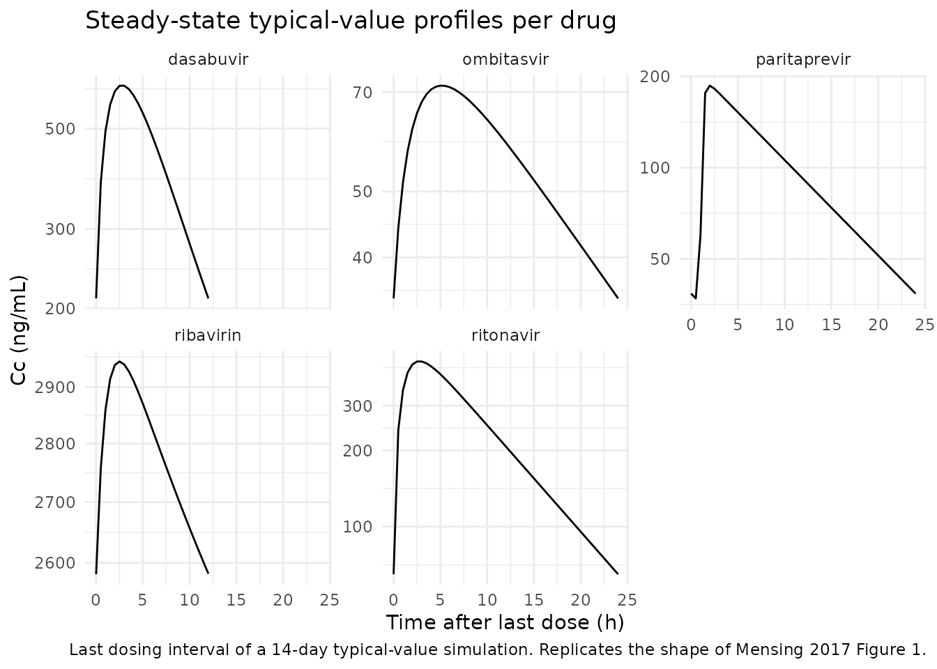
PKNCA validation
Steady-state NCA over the last dosing interval gives Cmax,ss, Tmax,ss, and AUC0-tau,ss. The independent validation check is that AUC0-24,ss should equal the total daily dose divided by the published CL/F (since at steady state, total input over 24 h equals total clearance x AUC0-24,ss). This holds for any dosing interval that adds up to 24 h of total exposure.
# Helper to extract the last dosing interval's NCA for a drug
nca_one_drug <- function(sim, dose_mg, tau_day, drug_label, conc_unit = "ug/mL") {
  end_time <- max(sim$time)
  start_ss <- end_time - tau_day

  # Concentration data over the last dosing interval; PKNCA needs the time-0
  # row, so anchor at t = start_ss with Cc(start_ss).
  sim_nca <- sim |>
    dplyr::filter(!is.na(Cc), time >= start_ss) |>
    dplyr::mutate(t_in_interval = time - start_ss) |>
    dplyr::select(id, time = t_in_interval, Cc)
  # Add a t = 0 row (the trough at the time of dose) if not already present.
  sim_nca <- dplyr::bind_rows(
    sim_nca,
    sim_nca |> dplyr::distinct(id) |>
      dplyr::mutate(time = 0, Cc = min(sim_nca$Cc[sim_nca$time == min(sim_nca$time)]))
  ) |>
    dplyr::distinct(id, time, .keep_all = TRUE) |>
    dplyr::arrange(id, time)

  dose_df <- data.frame(id = 1L, time = 0, amt = dose_mg)

  conc_obj <- PKNCA::PKNCAconc(sim_nca, Cc ~ time | id,
                               concu = conc_unit, timeu = "day")
  dose_obj <- PKNCA::PKNCAdose(dose_df, amt ~ time | id, doseu = "mg")

  intervals <- data.frame(
    start    = 0,
    end      = tau_day,
    cmax     = TRUE,
    tmax     = TRUE,
    auclast  = TRUE,
    cav      = TRUE
  )

  res <- PKNCA::pk.nca(PKNCA::PKNCAdata(conc_obj, dose_obj, intervals = intervals))
  out <- as.data.frame(res$result)
  out$drug <- drug_label
  out
}

nca_results <- list()
for (i in seq_len(nrow(drug_specs))) {
  drug <- drug_specs$drug[i]
  nca_results[[drug]] <- nca_one_drug(
    sim       = sims[[drug]],
    dose_mg   = drug_specs$dose_mg[i],
    tau_day   = drug_specs$tau_day[i],
    drug_label = drug
  )
}
nca_all <- dplyr::bind_rows(nca_results)

nca_wide <- nca_all |>
  dplyr::select(drug, PPTESTCD, PPORRES) |>
  tidyr::pivot_wider(names_from = PPTESTCD, values_from = PPORRES)

knitr::kable(nca_wide,
             caption = "Steady-state NCA per drug over one dosing interval (units: ug/mL for Cmax/Cav/Ctau, ug*day/mL for AUC, day for time).",
digits = 4)| drug | auclast | cmax | tmax | cav |
|---|---|---|---|---|
| paritaprevir | 0.0947 | 0.1865 | 0.0833 | 0.0947 |
| ombitasvir | 0.0552 | 0.0716 | 0.2083 | 0.0552 |
| ritonavir | 0.2274 | 0.4483 | 0.1250 | 0.2274 |
| dasabuvir | 0.2170 | 0.6225 | 0.1250 | 0.4339 |
| ribavirin | 1.3937 | 2.9464 | 0.1042 | 2.7875 |
Independent cross-check: AUC0-24,ss vs published CL/F
At steady state, the total daily input dose D_day equals the total amount cleared over 24 h, so AUC0-24,ss = D_day / (CL/F). For QD dosing (tau = 1 day), AUC0-tau,ss = AUC0-24,ss; for BID dosing (tau = 0.5 day), AUC0-24,ss is twice AUC0-tau,ss.
cl_pub <- tibble::tribble(
  ~drug,           ~cl_L_per_day,
  "paritaprevir",  1580,
  "ombitasvir",     453,
  "ritonavir",      439,
  "dasabuvir",     1150,
  "ribavirin",      427
)

auc_check <- nca_wide |>
  dplyr::left_join(drug_specs, by = "drug") |>
  dplyr::left_join(cl_pub, by = "drug") |>
  dplyr::mutate(
    auc_per_dose_simulated  = auclast / dose_mg,          # ug*day/mL per mg
    auc_per_dose_predicted  = 1 / cl_L_per_day,            # 1/(L/day) = day/L = ug*day/mL per mg (since 1 mg/L = 1 ug/mL)
    pct_difference          = 100 * (auc_per_dose_simulated - auc_per_dose_predicted) / auc_per_dose_predicted
  ) |>
  dplyr::select(drug, dose_mg, tau_day, cl_L_per_day,
                auc_per_dose_simulated, auc_per_dose_predicted, pct_difference)

knitr::kable(auc_check,
             caption = "Independent check: simulated AUC0-tau,ss per mg dose vs the published CL/F (auc_per_dose = 1 / CL/F at steady state).",
digits = 6)| drug | dose_mg | tau_day | cl_L_per_day | auc_per_dose_simulated | auc_per_dose_predicted | pct_difference |
|---|---|---|---|---|---|---|
| paritaprevir | 150 | 1.0 | 1580 | 0.000631 | 0.000633 | -0.243708 |
| ombitasvir | 25 | 1.0 | 453 | 0.002207 | 0.002208 | -0.037656 |
| ritonavir | 100 | 1.0 | 439 | 0.002274 | 0.002278 | -0.183969 |
| dasabuvir | 250 | 0.5 | 1150 | 0.000868 | 0.000870 | -0.202389 |
| ribavirin | 600 | 0.5 | 427 | 0.002323 | 0.002342 | -0.812910 |
Each row’s pct_difference should be close to 0 because
the steady-state relationship Dose = CL/F * AUC0-tau,ss must hold at
convergence. Larger deviations would point to either a transcription
error in CL/F or an incomplete-burn-in (the 14-day horizon not actually
reaching steady state for a slowly-eliminated drug; ribavirin in
particular has a multi-week distribution-phase half-life).
Assumptions and deviations
-
Covariate coefficients omitted. Mensing 2017’s
final models retain several significant covariates per drug on CL/F and
Vc/F (per Table 3): paritaprevir (cirrhosis, sex, age, opioid use,
antidiabetic use), ombitasvir (cirrhosis, sex, age, weight), dasabuvir
(cirrhosis, sex, CrCL, weight, age), ritonavir (sex, CrCL, HCV
genotype), ribavirin (cirrhosis, sex, CrCL). The paper publishes only
Figure 2 exposure-ratio forest plots (with 95% CIs) for each covariate;
coefficient point estimates are not reported in the main article or in
the named supplementary tables (S1-S5 contain only P-values per the
Supporting Information index). The implemented models are therefore the
structural typical-value models without covariate effects. The retained
covariates per drug are documented in each model’s
covariatesDataExcludedlist to preserve the provenance. Users who need the covariate-corrected model must back-derive the coefficients from Figure 2 (binary covariates: one exposure ratio gives one coefficient; continuous covariates: two exposure ratios at two values give two equations for the power exponents on CL/F and Vc/F). - Ribavirin correlated IIV not encoded. Mensing 2017 Results states “correlated IIV on CL/F and Vc/Vp” for ribavirin but Table 3 does not list the correlation value. The model encodes the random effects as independent.
-
Ribavirin shared IIV on Vc/F + Vp/F. Mensing 2017
reports a single IIV value (0.197) for both Vc/F and Vp/F. The model
applies the same eta (
etalvc) to both compartments so individuals with a larger central volume also have a proportionally larger peripheral volume. -
Paritaprevir lnorm residual error. The paper
reports an “additive error model on log-transformed data” which in
nlmixr2 maps to
Cc ~ lnorm(expSd)whereexpSdis the SD on the log scale. NONMEM reports variance (1.14), converted to SD assqrt(1.14) = 1.068for the nlmixr2 ini() value. -
Concentration units. The Mensing 2017 Methods
report LLOQ in ng/mL while Figure 1 axes are labelled
mg/mL. The latter is incompatible with the former by a factor of 10^9; the most plausible interpretation is that Figure 1’s axis label is a typo forug/mL(= mg/L). The model files useunits = list(time = "day", dosing = "mg", concentration = "ug/mL")and the vignette multiplies by 1000 to display ng/mL when plotting. - Dose used for ribavirin simulation. Ribavirin is administered at 600 mg twice daily (1200 mg/day) for body weight >= 75 kg, or 500 mg twice daily (1000 mg/day) for body weight < 75 kg. The simulation uses the heavier- weight regimen (600 mg BID) as the typical-value case; the cohort median weight for the ribavirin pharmacokinetic dataset is 77 kg (Mensing 2017 Table 2, ribavirin pharmacokinetic data column).