Sodium zirconium cyclosilicate and potassium homeostasis QSP (Clegg 2024)
Source:vignettes/articles/Clegg_2024_sodiumZirconiumCyclosilicate.Rmd
Clegg_2024_sodiumZirconiumCyclosilicate.RmdModel and source
mod_fun <- readModelDb("Clegg_2024_sodiumZirconiumCyclosilicate")
mod <- rxode2::rxode2(mod_fun)
meta <- mod_fun()- Citation: Clegg LE, Chu L, Nagard M, Boulton DW, Penland RC. Potassium homeostasis and therapeutic intervention with sodium zirconium cyclosilicate: A model-informed drug development case study. CPT Pharmacometrics Syst Pharmacol. 2024;13(2):296-307. doi:10.1002/psp4.13084
- Description: QSP. Four-compartment potassium-homeostasis model (gastrointestinal tract, blood, tissue extracellular fluid, tissue intracellular space) with reversible potassium binding to orally administered sodium zirconium cyclosilicate (SZC) in the gastrointestinal lumen, faecal loss of free and bound SZC, and eGFR-scaled renal potassium clearance with a sinusoidal diurnal rhythm, in adults with hyperkalaemia (Clegg 2024). An optional hemodialysis extension removes blood potassium into a fixed-concentration dialysate bath during sessions. Typical-value model: parameters are the medians of the per-subject fits; there is no IIV or residual error.
- Article: https://doi.org/10.1002/psp4.13084 (open access; Appendix S1 holds Table S1, Table S2 and the K+-SZC binding fit of Figure S2)
Clegg 2024 built a fit-for-purpose systems-pharmacology model of potassium (K+) homeostasis to support development of sodium zirconium cyclosilicate (SZC), a non-absorbed oral K+ binder. Potassium moves between four well-mixed compartments: the lumped gastrointestinal (GI) tract, blood (plasma / serum), tissue extracellular fluid and the tissue intracellular space. It enters with meals, is lost in faeces from the GI tract and through the kidneys from blood, and binds reversibly to SZC in the GI tract. Free and bound SZC leave in faeces at the same rate. Renal clearance scales with eGFR and follows a sinusoidal diurnal rhythm.
The model was fitted subject by subject (least squares with physiological penalties) to serum K+ (sK+) from the phase III trials ZS-003 and ZS-004, which gave a virtual population of 820 parameter sets. That population was then adapted to two applications: emergency treatment of severe hyperkalaemia (ENERGIZE design) and K+ control between hemodialysis sessions (DIALIZE design). The packaged model carries the median of each per-subject parameter (Clegg 2024 Table 1) as a typical-value model.
Structure
data.frame(
  state = mod$state,
  holds = c(
    "K+ in the GI tract (mmol)",
    "K+ in blood / serum (mmol)",
    "K+ in tissue extracellular fluid (mmol)",
    "K+ in the tissue intracellular space (mmol)",
    "free SZC in the GI tract (g)",
    "K+-SZC complex in the GI tract (mmol)"
  )
) |>
knitr::kable(caption = "Model states (all amounts).")| state | holds |
|---|---|
| gi_k | K+ in the GI tract (mmol) |
| blood_k | K+ in blood / serum (mmol) |
| tissue_ecf_k | K+ in tissue extracellular fluid (mmol) |
| tissue_icf_k | K+ in the tissue intracellular space (mmol) |
| gi_szc | free SZC in the GI tract (g) |
| gi_kszc | K+-SZC complex in the GI tract (mmol) |
Doses go into gi_szc for SZC (amount in grams) and into
gi_k for dietary K+ (amount in mmol, which equals mEq for a
monovalent ion). Model time 0 must be a midnight,
because the diurnal factor m(t) = 1 - p * cos(pi * t / 12)
is written in clock time (lowest at midnight, highest at noon).
Population
The model was developed on 820 adults with hyperkalaemia whose per-subject fits were accepted: 652 of 753 from ZS-003 (sK+ 5-6.5 mmol/L at entry) and 168 of 258 from ZS-004 / HARMONIZE (sK+ >= 5.1 mmol/L). Mean age was 65.3 (SD 12.2) years and mean weight 89.2 (SD 22.0) kg. 61% were male, 84% White, 13% Black or African American and 3% other races. Mean eGFR was 44.1 (SD 25.3) mL/min/1.73 m^2. 55% had chronic kidney disease, 43% type 2 diabetes and 10% congestive heart failure, and 42% took an ACE inhibitor (Clegg 2024 Table S2). In both trials, SZC (1.25-10 g) or placebo was given three times daily for 48 h (acute phase). Maintenance followed with once-daily dosing (ZS-003: same dose or placebo for 12 days; ZS-004: 0, 5, 10 or 15 g for 28 days).
The same information is available programmatically via
meta$population.
Source trace
Every ini() value carries an in-file comment naming its
source. The table collects them.
| Parameter / equation | Value | Source location |
|---|---|---|
lr_gb (r_GB) |
log(0.062) 1/h | Table 1, median (IQR 0.041, 0.11) |
lr_bg (r_BG) |
log(0.23) 1/h | Table 1, median (IQR 0.09, 3.8) |
lr_eb (r_EB) |
log(3.9) 1/h | Table 1, median (IQR 0.14, 49.9) |
r_be_eb (r_BE = 2.3 r_EB) |
2.3 | Table 1 r_BE row; Methods (“r_BE = 2.3 x r_EB”) |
lr_ei (r_EI) |
log(0.091) 1/h | Table 1, median (IQR 0.069, 0.12) |
lr_ie (r_IE) |
log(0.0011) 1/h | Table 1, median (IQR 0.00083, 0.0015) |
lr_cl_k (r_CL,K) |
log(0.0065) 1/h | Table 1, median (IQR 0.0036, 0.011) |
lr_cl_szc (r_CL,SZC) |
log(0.42) 1/h | Table 1, median (IQR 0.26, 0.79) |
lr_renal (r_renal) |
log(0.18) 1/h | Table 1, median (IQR 0.13, 0.29) |
p_diurnal (p) |
0.20 | Table 1, median (IQR 0.073, 0.49) |
lr_on (r_on) |
log(1503.36) 1/(mM h) | Figure S2c small-intestine k_on 69.6 /(M s), x 3.6 for units, x 6 in vivo (Methods; Figure 2) |
lr_off (r_off) |
log(7704) 1/h | Figure S2c small-intestine k_off 2.14 /s |
mw_szc |
410 g/mol | Figure S2 legend (“ZS-9 molecular weight of 410 g/mol”) |
f_vb |
0.048 L/kg | Table S1 (20% of ECF, 40% of TBW, 60% of weight); Figure 1 |
f_ve |
0.110769 L/kg | Table S1 (8/13 of TIF, 75% of ECF) |
f_vi |
0.36 L/kg | Table S1 (60% of TBW); Figure 1 |
vgi |
3 L | Table S1; Figure 1; Methods |
k_intake |
100 mmol/day | Methods, Information sources |
lr_d (r_D) |
log(1.05) 1/h | Figure 5 flow chart |
k_dialysate |
2 mmol/L | Results; Figure 5 flow chart |
d/dt(gi_k), d/dt(blood_k),
d/dt(tissue_ecf_k), d/dt(tissue_icf_k)
|
n/a | Model equations, Potassium homeostasis |
d/dt(gi_szc), d/dt(gi_kszc)
|
n/a | Model equations, SZC equations |
m(t) |
n/a | Model equations; Model equations text (maximum at noon) |
| initial conditions | n/a | Figure S1 steady-state equations |
| dialysis flux, fixed intracellular K+ | n/a | Figure 1 dialysis bath; Figure 5 flow chart; Results |
Dimensional analysis
The paper writes its equations in concentrations (mM). The packaged
model multiplies each equation by its compartment volume, so every state
is an amount and every term below is in mmol/h, except
gi_szc, which is in g/h.
| Term | Units |
|---|---|
r_gb * gi_k, r_bg * blood_k,
r_eb * tissue_ecf_k, r_be * blood_k, … |
1/h x mmol = mmol/h |
r_f * m(t) * blood_k, with
r_f = r_renal * eGFR / 60
|
1/h x (mL/min/1.73 m^2 / mL/min/1.73 m^2) x mmol = mmol/h |
bind = (r_on * k_gi * szc_gi - r_off * kszc_gi) * vgi |
(1/(mM h) x mM x mM - 1/h x mM) x L = mmol/h |
szc_gi = gi_szc / mw_szc * 1000 / vgi |
g / (g/mol) x (mmol/mol) / L = mM |
bind * mw_szc / 1000 in d/dt(gi_szc)
|
mmol/h x g/mol / (mmol/mol) = g/h |
RRT_HEMODIAL_ACTIVE * r_d * (k_b - k_dialysate) * vb |
1/h x mM x L = mmol/h |
Shared helpers
typ_wt <- 89.19 # Table S2 combined mean weight (kg)
typ_egfr <- 44.11 # Table S2 combined mean eGFR (mL/min/1.73 m^2)

# Meals: 100 mmol K+/day, 25% at 8 AM, 33% at noon, 42% at 6 PM (Methods).
meal_events <- function(ndays) {
  tidyr::expand_grid(day = seq_len(ndays) - 1, slot = 1:3) |>
    mutate(
      time = day * 24 + c(8, 12, 18)[slot],
      amt = c(25, 33, 42)[slot],
      cmt = "gi_k",
      evid = 1L
    ) |>
    select(time, amt, cmt, evid)
}

# One subject's event table: meals, optional SZC doses (time, amt in g),
# observations of serum K+ on the blood_k state, and covariate columns.
make_events <- function(ndays, szc = NULL, id = 1L, wt = typ_wt,
                        egfr = typ_egfr, hd_status = 0L, hd_days = NULL,
                        dt = 0.5) {
  obs <- data.frame(
    time = seq(0, ndays * 24, by = dt),
    amt = 0,
    cmt = "blood_k",
    evid = 0L
  )
  szc_ev <- if (is.null(szc) || nrow(szc) == 0L) {
    NULL
  } else {
    data.frame(time = szc$time, amt = szc$amt, cmt = "gi_szc", evid = 1L)
  }
  ev <- bind_rows(meal_events(ndays), szc_ev, obs) |>
    arrange(time, desc(evid))
  hd_on <- rep(0L, nrow(ev))
  for (d in hd_days) {
    hd_on[ev$time >= d * 24 + 8 & ev$time < d * 24 + 12] <- 1L
  }
  ev |>
    mutate(
      id = id,
      WT = wt,
      CRCL = egfr,
      RRT_HEMODIAL_ACTIVE = hd_on,
      RRT_HEMODIAL_STATUS = hd_status
    )
}
Steady state and mass balance
With a constant K+ intake and no diurnal rhythm
(p_diurnal = 0), the Figure S1 initial conditions are the
exact steady state, so the solution must not move.
mod_flat <- mod_fun |> rxode2::ini(p_diurnal = 0)
#> ℹ change initial estimate of `p_diurnal` to `0`
ev_ss <- data.frame(
  id = 1L, time = c(0, seq(0, 20 * 24, by = 6)),
  amt = c(100 * 20, rep(0, 81)), rate = c(100 / 24, rep(0, 81)),
  cmt = c("gi_k", rep("blood_k", 81)), evid = c(1L, rep(0L, 81)),
  WT = typ_wt, CRCL = typ_egfr, RRT_HEMODIAL_ACTIVE = 0L,
  RRT_HEMODIAL_STATUS = 0L
)
sim_ss <- rxode2::rxSolve(mod_flat, events = ev_ss) |> as.data.frame()
drift <- max(abs(sim_ss$Cc / sim_ss$Cc[1] - 1))
c(sK_mmol_L = sim_ss$Cc[1], max_relative_drift = drift)
#>          sK_mmol_L max_relative_drift
#>           5.714462           0.000000
stopifnot(drift < 1e-4)
The same initial conditions give the K+ balance at steady state. Intake must equal renal plus faecal loss, and the physiological constraints imposed during fitting (Figure 1, top-left inset) should hold for the typical subject: at least 70% of K+ cleared by the kidneys, intracellular K+ 120-150 mM, and extracellular K+ close to plasma K+.
th <- as.list(meta$theta)
p <- with(th, list(
  r_gb = exp(lr_gb), r_bg = exp(lr_bg), r_eb = exp(lr_eb),
  r_ei = exp(lr_ei), r_ie = exp(lr_ie), r_cl_k = exp(lr_cl_k),
  r_f = exp(lr_renal) * typ_egfr / 60, r_be_eb = r_be_eb,
  vb = f_vb * typ_wt, ve = f_ve * typ_wt, vi = f_vi * typ_wt,
  r_in = k_intake / 24
))
bal <- with(p, {
  kb <- (r_in / vb * r_gb / (r_cl_k + r_gb)) /
    (r_bg + r_f - r_gb * r_bg / (r_cl_k + r_gb))
  a_gi <- (r_in + r_bg * vb * kb) / (r_cl_k + r_gb)
  ke <- kb * r_be_eb * vb / ve
  ki <- ke * r_ei / r_ie * ve / vi
  data.frame(
    plasma_K_mM = kb, extracellular_K_mM = ke, intracellular_K_mM = ki,
    intake_mmol_h = r_in, renal_mmol_h = r_f * kb * vb,
    faecal_mmol_h = r_cl_k * a_gi,
    renal_fraction = r_f * kb * vb / r_in
  )
})
knitr::kable(t(signif(bal, 4)), col.names = "Typical subject")| Typical subject | |
|---|---|
| plasma_K_mM | 5.7140 |
| extracellular_K_mM | 5.6950 |
| intracellular_K_mM | 145.0000 |
| intake_mmol_h | 4.1670 |
| renal_mmol_h | 3.2370 |
| faecal_mmol_h | 0.9293 |
| renal_fraction | 0.7770 |
stopifnot(
  abs(bal$renal_mmol_h + bal$faecal_mmol_h - bal$intake_mmol_h) < 1e-9,
  bal$renal_fraction >= 0.70,
  bal$intracellular_K_mM > 120, bal$intracellular_K_mM < 150,
  abs(bal$extracellular_K_mM / bal$plasma_K_mM - 1) < 0.01
)
The ratio r_BE / r_EB = 2.3 is the ratio of the tissue-extracellular to blood volume (0.110769 / 0.048 = 2.31), which is why extracellular and plasma K+ come out equal at steady state, as the Methods state.
Diurnal profile (Figure 1 inset)
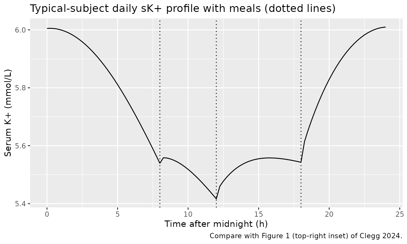
With three meals a day, the typical subject settles into a daily cycle. sK+ peaks near midnight, when renal clearance is lowest, and dips after breakfast.
sim_day <- rxode2::rxSolve(mod, events = make_events(5, dt = 0.25)) |>
  as.data.frame() |>
  filter(time >= 72, time <= 96) |>
  mutate(clock = time - 72)

ggplot(sim_day, aes(clock, Cc)) +
  geom_line() +
  geom_vline(xintercept = c(8, 12, 18), linetype = "dotted") +
  labs(
    x = "Time after midnight (h)", y = "Serum K+ (mmol/L)",
    title = "Typical-subject daily sK+ profile with meals (dotted lines)",
    caption = "Compare with Figure 1 (top-right inset) of Clegg 2024."
  )
day_summary <- data.frame(
  at_midnight = sim_day$Cc[sim_day$clock == 0],
  at_8am = sim_day$Cc[sim_day$clock == 8],
  daily_variation_pct = 100 * diff(range(sim_day$Cc)) / mean(sim_day$Cc)
)
knitr::kable(signif(day_summary, 3))| at_midnight | at_8am | daily_variation_pct |
|---|---|---|
| 6 | 5.54 | 10.4 |
# Fits with diurnal variation below 1.7% or above 15% were screened out of the
# virtual population (Methods), so the typical subject must fall inside it.
stopifnot(
  day_summary$daily_variation_pct > 1.7,
  day_summary$daily_variation_pct < 15,
  day_summary$at_midnight > day_summary$at_8am
)
The virtual population’s simulated mean sK+ was 5.17 mmol/L at 8 AM and 5.59 mmol/L at midnight (Table S2). The typical subject, built from the median of each parameter, sits about 0.4 mmol/L higher at both times, but the 8 AM-to-midnight rise of 0.4-0.5 mmol/L is reproduced. The median of each parameter need not give the population-mean output, because sK+ is a nonlinear function of the parameters.
ZS-004 dose response (Figure 3, right)
ZS-004 / HARMONIZE gave SZC 10 g three times daily for 48 h, then 0 (placebo), 5, 10 or 15 g once daily for 28 days. The simulation runs in for 3 days on meals alone, then gives the acute doses with meals (8 AM, noon, 6 PM) and the maintenance doses at 8 AM. Time is shown in days from the midnight before the first dose, as in the paper.
runin <- 3
zs004 <- function(maint_g) {
  acute <- data.frame(
    time = as.vector(outer(c(8, 12, 18), (runin + 0:1) * 24, "+")),
    amt = 10
  )
  maint <- data.frame(time = (runin + 2:29) * 24 + 8, amt = maint_g)
  bind_rows(acute, filter(maint, amt > 0))
}
arms <- c(0, 5, 10, 15)
ev_zs004 <- bind_rows(lapply(seq_along(arms), function(i) {
  make_events(runin + 37, szc = zs004(arms[i]), id = i, dt = 1) |>
    mutate(arm = paste0("Maintenance: ", ifelse(arms[i] == 0, "Placebo", paste(arms[i], "g"))))
}))
sim_zs004 <- rxode2::rxSolve(mod, events = ev_zs004, keep = "arm") |>
  as.data.frame() |>
  mutate(day = time / 24 - runin)

ggplot(filter(sim_zs004, day >= -1), aes(day, Cc)) +
  geom_line(colour = "purple4") +
  facet_wrap(~arm) +
  annotate("rect", xmin = 0, xmax = 2, ymin = -Inf, ymax = Inf, alpha = 0.1, fill = "blue") +
  annotate("rect", xmin = 2, xmax = 30, ymin = -Inf, ymax = Inf, alpha = 0.08, fill = "orange") +
  labs(
    x = "Time (days)", y = "Serum K+ (mmol/L)",
    title = "ZS-004: acute 10 g TID, then once-daily maintenance (typical subject)",
    caption = "Replicates Figure 3 (right) of Clegg 2024; shading marks the acute (blue) and maintenance (orange) periods."
  )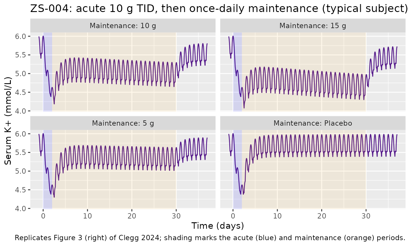
Clinical sK+ was mostly measured at 8 AM, before the daily dose. The table compares the typical-subject 8 AM values with the observed arm means read from Figure 3 (right) by the maintainers.
at8 <- function(d) sim_zs004 |> filter(abs(day - (d + 8 / 24)) < 1e-6)
zs004_tab <- bind_rows(
  at8(0) |> mutate(when = "Day 0, 8 AM (baseline)"),
  at8(2) |> mutate(when = "Day 2, 8 AM (end of acute phase)"),
  at8(15) |> mutate(when = "Day 15, 8 AM (maintenance)"),
  at8(29) |> mutate(when = "Day 29, 8 AM (end of maintenance)")
) |>
  select(arm, when, Cc) |>
  mutate(Cc = round(Cc, 2)) |>
  pivot_wider(names_from = arm, values_from = Cc)
knitr::kable(zs004_tab, caption = "Typical-subject sK+ (mmol/L) by ZS-004 arm.")| when | Maintenance: Placebo | Maintenance: 5 g | Maintenance: 10 g | Maintenance: 15 g |
|---|---|---|---|---|
| Day 0, 8 AM (baseline) | 5.54 | 5.54 | 5.54 | 5.54 |
| Day 2, 8 AM (end of acute phase) | 4.38 | 4.38 | 4.38 | 4.38 |
| Day 15, 8 AM (maintenance) | 5.51 | 5.26 | 5.03 | 4.80 |
| Day 29, 8 AM (end of maintenance) | 5.51 | 5.23 | 4.95 | 4.68 |
observed_fig3 <- data.frame(
  arm = c("Placebo", "5 g", "10 g", "15 g"),
  baseline = c(5.7, 5.5, 5.5, 5.5),
  end_acute = c(4.6, 4.5, 4.4, 4.4),
  maintenance = c(5.3, 4.8, 4.5, 4.4)
)
knitr::kable(observed_fig3, caption = "Observed ZS-004 arm means read from Figure 3 (right) of Clegg 2024 (approximate, mmol/L).")| arm | baseline | end_acute | maintenance |
|---|---|---|---|
| Placebo | 5.7 | 4.6 | 5.3 |
| 5 g | 5.5 | 4.5 | 4.8 |
| 10 g | 5.5 | 4.4 | 4.5 |
| 15 g | 5.5 | 4.4 | 4.4 |
d0 <- at8(0)$Cc
d2 <- at8(2)$Cc
d15 <- at8(15)$Cc
stopifnot(
  # 48 h of 10 g TID lowers sK+ by about 1 mmol/L (observed ~1.0-1.1).
  all(d0 - d2 > 0.6), all(d0 - d2 < 1.6),
  # Maintenance response rises with dose (deterministic, typical subject).
  all(diff(d15) < 0)
)
During the acute phase the typical subject falls by 1.16 mmol/L, against about 1.0-1.1 mmol/L in the observed means. Its 8 AM baseline matches the observed arm means. Maintenance separates the arms in dose order, as observed, but the typical subject sits 0.2-0.5 mmol/L above the observed arm means. Its placebo-to-15 g spread is about 0.7 mmol/L, against about 0.9 mmol/L observed. The paper’s own population simulation (Figure 3) tracks the observed means more closely, because the population mean is not the response of a median subject. After the last dose the simulated subjects drift back toward their baseline over days; the paper notes this as a property of the model’s structure.
Emergency treatment of severe hyperkalaemia (Figure 4)
For the ENERGIZE design, Clegg 2024 lowered r_renal by 15% in every virtual subject to raise baseline sK+ to the trial’s mean (6.41 mmol/L simulated, 6.38 observed). They then kept the subjects with sK+ >= 5.8 mmol/L. Baseline was assumed at 8 PM, and SZC was given as 10 g at 1, 4 and 10 h, 30 g at 1 h, or 60 g at 1 h. The same r_renal reduction is applied to the typical subject.
mod_er <- mod_fun |> rxode2::ini(lr_renal = log(0.18 * 0.85))
#> ℹ change initial estimate of `lr_renal` to `-1.8773173575897`
bl_time <- runin * 24 + 20 # 8 PM on the third day
regimens <- list(
  "Placebo" = NULL,
  "SZC 10 g x 3" = data.frame(time = bl_time + c(1, 4, 10), amt = 10),
  "SZC 30 g x 1" = data.frame(time = bl_time + 1, amt = 30),
  "SZC 60 g x 1" = data.frame(time = bl_time + 1, amt = 60)
)
ev_er <- bind_rows(lapply(seq_along(regimens), function(i) {
  make_events(runin + 2, szc = regimens[[i]], id = i, dt = 0.25) |>
    mutate(regimen = names(regimens)[i])
}))
sim_er <- rxode2::rxSolve(mod_er, events = ev_er, keep = "regimen") |>
  as.data.frame() |>
  mutate(tad = time - bl_time - 1) |>
  group_by(regimen) |>
  mutate(cfb = Cc - Cc[abs(time - bl_time) < 1e-6]) |>
  ungroup()

ggplot(filter(sim_er, tad >= -4, tad <= 32), aes(tad, Cc, colour = regimen)) +
  geom_line() +
  geom_vline(xintercept = 4, linetype = "dashed") +
  geom_hline(yintercept = 5.5, linetype = "dashed") +
  labs(
    x = "Time after first SZC dose (h)", y = "Serum K+ (mmol/L)", colour = NULL,
    title = "Emergency dosing, typical subject with r_renal lowered 15%",
    caption = "Replicates Figure 4 (bottom) of Clegg 2024."
  )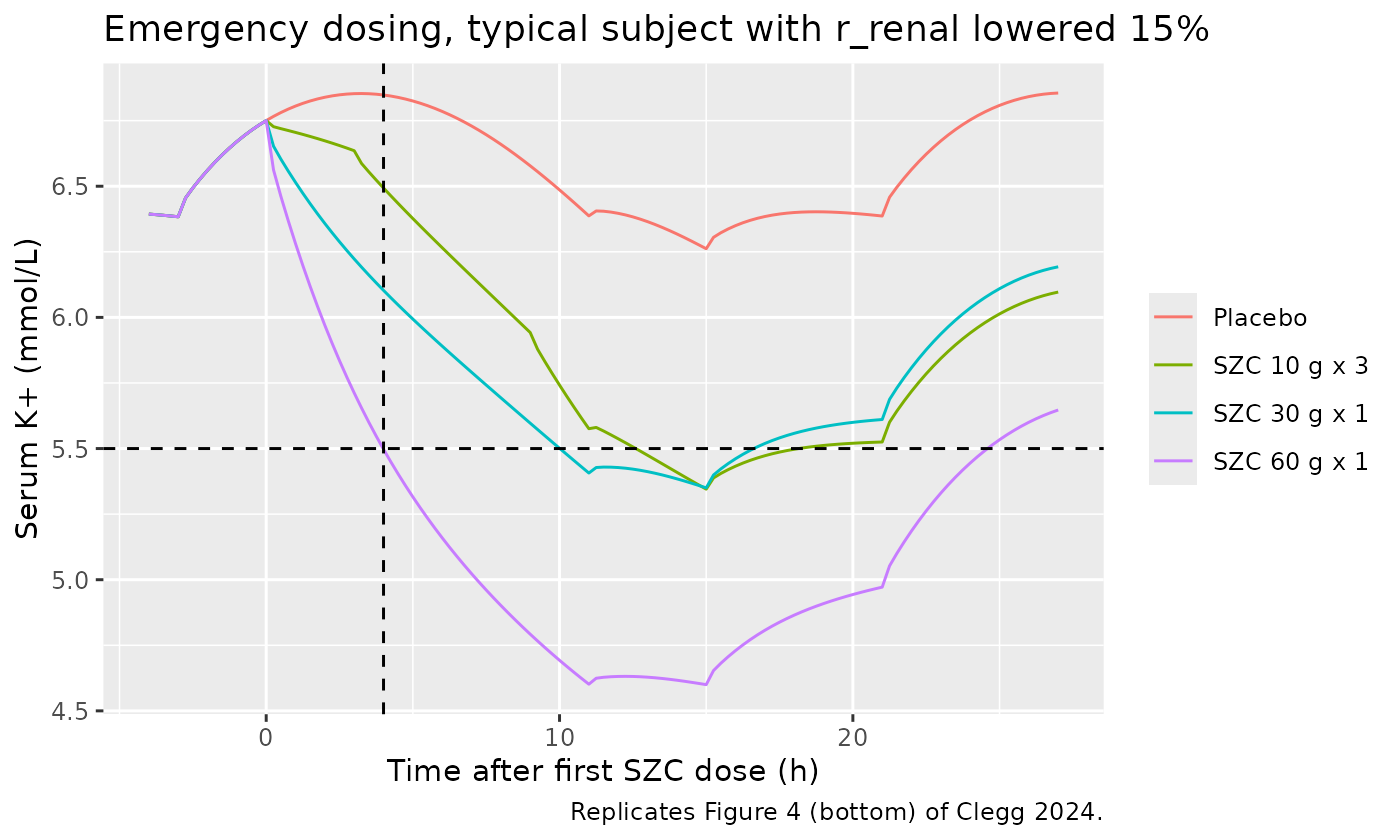
The primary end point of ENERGIZE was the change in sK+ from baseline to 4 h after the first dose (Figure 2), marked by the vertical dashed line in Figure 4. The maintainers read the population-mean change from baseline at that line from Figure 4.
cfb4 <- sim_er |>
  filter(abs(tad - 4) < 1e-6) |>
  select(regimen, Cc, cfb) |>
  mutate(figure_4 = c(0.05, -0.3, -0.65, -1.2)[match(regimen, names(regimens))])
placebo_cfb <- cfb4$cfb[cfb4$regimen == "Placebo"]
cfb4 |>
  mutate(placebo_corrected = cfb - placebo_cfb) |>
  mutate(across(where(is.numeric), \(x) round(x, 2))) |>
  rename(
    "Regimen" = regimen,
    "sK+ at 4 h (mmol/L)" = Cc,
    "Change from baseline" = cfb,
    "Figure 4 mean change from baseline (approx.)" = figure_4,
    "Placebo-corrected change" = placebo_corrected
  ) |>
knitr::kable(caption = "Change in sK+ (mmol/L) 4 h after the first SZC dose.")| Regimen | sK+ at 4 h (mmol/L) | Change from baseline | Figure 4 mean change from baseline (approx.) | Placebo-corrected change |
|---|---|---|---|---|
| Placebo | 6.85 | 0.18 | 0.05 | 0.00 |
| SZC 10 g x 3 | 6.49 | -0.18 | -0.30 | -0.35 |
| SZC 30 g x 1 | 6.10 | -0.57 | -0.65 | -0.74 |
| SZC 60 g x 1 | 5.50 | -1.17 | -1.20 | -1.35 |
# Typical-subject changes were within 0.13 mmol/L of the Figure 4 readings
# (largest gap: placebo, +0.18 vs +0.05). A transcription error in the binding
# constants, the SZC mass-to-moles conversion or the GI volume moves the 60 g
# change by far more than 0.35 mmol/L.
stopifnot(all(abs(cfb4$cfb - cfb4$figure_4) < 0.35))
The typical subject reproduces the paper’s conclusion. 10 g x 3 changes sK+ only modestly within 4 h, and 30 g falls well short of the 1 mmol/L drop that a mean baseline of 6.4 mmol/L needs to get below 5.5 mmol/L. Only 60 g reaches it. The typical baseline (6.67 mmol/L) is higher than the population mean (see above), so even with 60 g its absolute 4-h value only just reaches 5.5 mmol/L. The comparison is therefore made on the change from baseline.
Hemodialysis (Figure 5)
For the DIALIZE design, Clegg 2024 kept the virtual subjects with
eGFR < 20 mL/min/1.73 m^2 and added a dialysis bath. During sessions
blood K+ transfers to a dialysate fixed at 2 mmol/L with r_D = 1.05 1/h.
Sessions ran Monday, Wednesday and Friday, 8 AM to noon. Intracellular
K+ was held at its steady-state value, and r_renal was lowered by 12% to
match the pre-dialysis sK+ in DIALIZE. In the packaged model,
RRT_HEMODIAL_ACTIVE = 1 switches the dialysis flux on
during a session, and RRT_HEMODIAL_STATUS = 1 holds
intracellular K+ at its initial steady state.
eGFR enters the model only through the product r_renal x eGFR / 60. The eGFR < 20 subjects were fitted to sK+ of 5-6 mmol/L, so their own r_renal values sit far above the population median. Pairing the median r_renal with eGFR 15 would describe a subject the model never fitted, with a no-dialysis steady-state sK+ well above 10 mmol/L. The maintainers therefore built a representative dialysis subject with eGFR 15 whose renal K+ clearance r_renal x eGFR / 60 equals that of the typical subject, and then applied the paper’s 12% reduction.
SZC 0 (placebo), 5, 10 or 15 g was given once daily at 8 AM on non-dialysis days. Doses were titrated up by 5 g per week to the target, then held for a 4-week evaluation period, as the paper assumed.
hd_egfr <- 15
mod_hd <- mod_fun |> rxode2::ini(lr_renal = log(0.18 * typ_egfr / hd_egfr * 0.88))
#> ℹ change initial estimate of `lr_renal` to `-0.763995486587173`
hd_weeks <- 2 + 8 # 2 weeks of dialysis run-in, 4 weeks titration, 4 weeks stable
hd_days <- as.vector(outer(c(0, 2, 4), 7 * (seq_len(hd_weeks) - 1), "+")) # Mon/Wed/Fri
non_hd <- setdiff(seq_len(hd_weeks * 7) - 1, hd_days)
hd_dose <- function(target_g) {
  week <- non_hd %/% 7 - 1 # SZC week 1 starts on day 14
  dose <- pmin(target_g, 5 * week)
  data.frame(time = non_hd * 24 + 8, amt = dose) |> filter(week >= 1, amt > 0)
}
targets <- c(0, 5, 10, 15)
ev_hd <- bind_rows(lapply(seq_along(targets), function(i) {
  make_events(hd_weeks * 7, szc = hd_dose(targets[i]), id = i,
    egfr = hd_egfr, hd_status = 1L, hd_days = hd_days, dt = 0.5) |>
    mutate(group = ifelse(targets[i] == 0, "Placebo", paste0("SZC ", targets[i], " g")))
}))
sim_hd <- rxode2::rxSolve(mod_hd, events = ev_hd, keep = "group") |>
  as.data.frame() |>
  mutate(
    day = time / 24,
    group = factor(group, levels = c("Placebo", "SZC 5 g", "SZC 10 g", "SZC 15 g"))
  )

last_week <- (hd_weeks - 1) * 7
ggplot(filter(sim_hd, day >= last_week), aes(day - last_week, Cc, colour = group)) +
  geom_line() +
  labs(
    x = "Time (days, Monday 0:00 of the last evaluation week)",
    y = "Serum K+ (mmol/L)", colour = NULL,
    title = "Hemodialysis Mon/Wed/Fri, SZC on non-dialysis days at 8 AM",
    caption = "Replicates Figure 5 (bottom right) of Clegg 2024 for a representative subject."
  )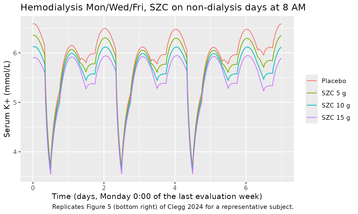
The paper compares pre- and post-dialysis sK+ after the last long interdialytic interval (LIDI, Friday to Monday) of the evaluation period with DIALIZE (Figure 5, middle right).
lidi_monday <- last_week
pre_post <- sim_hd |>
  filter(abs(time - (lidi_monday * 24 + 8)) < 1e-6 | abs(time - (lidi_monday * 24 + 12)) < 1e-6) |>
  mutate(when = ifelse(abs(time - lidi_monday * 24 - 8) < 1e-6, "pre", "post")) |>
  select(group, when, Cc) |>
  pivot_wider(names_from = when, values_from = Cc)
hd_tab <- pre_post |>
  mutate(
    dialize_pre = c(5.7, NA, NA, NA)[match(group, c("Placebo", "SZC 5 g", "SZC 10 g", "SZC 15 g"))],
    dialize_post = c(3.9, NA, NA, NA)[match(group, c("Placebo", "SZC 5 g", "SZC 10 g", "SZC 15 g"))]
  ) |>
  mutate(across(where(is.numeric), \(x) round(x, 2))) |>
  rename(
    "Group" = group,
    "Pre-dialysis sK+" = pre,
    "Post-dialysis sK+" = post,
    "DIALIZE placebo pre (approx.)" = dialize_pre,
    "DIALIZE placebo post (approx.)" = dialize_post
  )
knitr::kable(hd_tab, caption = "sK+ (mmol/L) around the dialysis session after the last LIDI.")| Group | Pre-dialysis sK+ | Post-dialysis sK+ | DIALIZE placebo pre (approx.) | DIALIZE placebo post (approx.) |
|---|---|---|---|---|
| Placebo | 6.14 | 3.73 | 5.7 | 3.9 |
| SZC 5 g | 5.96 | 3.67 | NA | NA |
| SZC 10 g | 5.77 | 3.60 | NA | NA |
| SZC 15 g | 5.60 | 3.54 | NA | NA |
stopifnot(
  # A 4-h session removes about 2 mmol/L (DIALIZE placebo: 5.7 -> 3.9).
  all(pre_post$pre - pre_post$post > 1.4), all(pre_post$pre - pre_post$post < 3),
  # Pre-dialysis sK+ falls with SZC dose.
  all(diff(pre_post$pre[match(c("Placebo", "SZC 5 g", "SZC 10 g", "SZC 15 g"), pre_post$group)]) < 0)
)
For DIALIZE, Figure 5 (middle right) shows the observed SZC-treated pre-dialysis mean near 5.1 mmol/L and the post-dialysis mean near 3.6 mmol/L. The paper’s population simulations gave a pre-dialysis mean of about 5.5 mmol/L with 5 g, 5.3 with 10 g and 5.1 with 15 g. For the representative subject the fall in pre-dialysis sK+ per dose step is similar. It starts from a placebo pre-dialysis value somewhat above the DIALIZE mean of 5.7 mmol/L, because its parameters were not tuned to the DIALIZE placebo arm the way the paper’s population was.
Assumptions and deviations
- Typical-value model. Clegg 2024 fitted each subject separately and did not estimate a population model. Table 1 reports only the median and IQR of the per-subject estimates, and the packaged model uses the medians. The paper states that means and a covariance matrix of the individual parameters were provided with an R script as File S1 in Appendix S1. The published Appendix S1 (Wiley and PubMed Central, checked 2026-10-29) contains only the Word document, so no between-subject variability is encoded and the model has no residual error (the fit was penalised least squares). The median of each parameter does not reproduce the population-mean sK+; the typical subject runs about 0.4 mmol/L above the Table S2 means.
- SZC dose to concentration. The equations do not state the units of the SZC state. The maintainers converted the SZC mass to moles of K+ binding sites with the 410 g/mol that Clegg 2024 used for the in vitro binding fit (Figure S2), with one K+ per site and the 3-L GI volume. This gives about 2.4 mmol K+ binding capacity per gram. The Figure 4 emergency-dosing changes and the ZS-004 48-h fall are reproduced to within about 0.1-0.2 mmol/L with this conversion.
- Tissue extracellular volume. Figure 1 labels the tissue extracellular compartment “18% of weight”, which is the whole tissue interstitial fluid of Table S1 (75% of ECF). Table S1 states that the model’s V_E is 8/13 of it, 0.110769 L/kg. The Table S1 value was used because the fixed ratio r_BE = 2.3 x r_EB is described as the volume ratio, and 0.110769 / 0.048 = 2.31 whereas 0.18 / 0.048 = 3.75.
- Renal clearance. The equation writes renal clearance as r_f, and Table 1 and Figure 1 call it r_renal. They were taken as the same parameter, multiplied by eGFR / 60 and m(t) as in the equation and Figure 1.
- Dialysis flux. Clegg 2024 describes a one-way transfer of K+ from blood to a dialysate bath at a fixed K+ concentration of 2 mmol/L. This was encoded as r_D x (K_B - 2 mmol/L), the form in which the dialysate concentration matters. The representative subject drops by about 2.4 mmol/L over a session, against about 1.8 mmol/L in the DIALIZE placebo arm.
-
Fixed intracellular K+ in hemodialysis. “Fix
intracellular K+ to steady-state value” (Figure 5) was encoded as a zero
derivative for the intracellular state whenever
RRT_HEMODIAL_STATUS = 1. The state then stays at its initial no-dialysis steady state for the whole simulation. - Dosing times. The paper used each subject’s dosing records and does not print the times of the three daily acute doses. The maintainers gave them with meals (8 AM, noon, 6 PM). Maintenance doses were given at 8 AM, as in the hemodialysis application.
- Initial conditions. The Figure S1 steady state under constant intake initialises every subject. A run-in of at least 48 h with meals then establishes the diurnal cycle before dosing, as in the paper (3 days used here).
-
Application adjustments. The 15% (emergency) and
12% (hemodialysis) reductions in r_renal, and the representative
dialysis subject’s r_renal, are made in this article with
rxode2::ini(). They are not built into the packaged model. - Observed values in the comparison tables were read from Figures 3, 4 and 5 by the maintainers and are approximate (about +/- 0.1 mmol/L).
- No correction notice for Clegg 2024 was found in Europe PMC (searches for corrections and the list of citing records) as of 2026-10-29.