Nintedanib (Schmid 2017) • nlmixr2lib

Model and source

Citation: Schmid U, Liesenfeld KH, Fleury A, Dallinger C, Freiwald M. Population pharmacokinetics of nintedanib, an inhibitor of tyrosine kinases, in patients with non-small cell lung cancer or idiopathic pulmonary fibrosis. Cancer Chemotherapy and Pharmacology. 2018 Jan;81(1):89-101. doi:10.1007/s00280-017-3452-0. PMID 29127500.
Article: https://doi.org/10.1007/s00280-017-3452-0 (open access, CC-BY 4.0)
Online Resource (supplement, Tables S1-S7, Figures S1-S6): retrieved from https://link.springer.com/article/10.1007/s00280-017-3452-0

The packaged model is a joint parent + metabolite popPK for nintedanib (a triple angiokinase inhibitor used in NSCLC and IPF) and its main hydrolytic metabolite BIBF 1202. The structural model is two parallel first-order-absorption + absorption-lag + one-compartment chains coupled by (1) a small first-pass formation of BIBF 1202 from the oral dose (relative bioavailability F2 = F1 * 0.0110) and (2) a slow systemic formation of BIBF 1202 from the nintedanib central compartment at rate kmet = CL/V2 * ffM (ffM = 0.000931, fixed).

Population

The population PK analysis pooled data from 1191 patients (5611 nintedanib and 5376 BIBF 1202 plasma concentrations) across four clinical trials:

TOMORROW (Richeldi 2011 NEJM): n = 342 IPF patients on nintedanib 50 mg QD, 50 mg BID, 100 mg BID, or 150 mg BID monotherapy over a 52-week period.
NSCLC Phase II (Reck 2011 Ann Oncol): n = 73 second-line NSCLC patients on nintedanib 150 or 250 mg BID monotherapy.
LUME-Lung 1 (Reck 2014 Lancet Oncol): n = 652 second-line NSCLC patients on nintedanib 200 mg BID + docetaxel 75 mg/m^2 q3w.
LUME-Lung 2 (Hanna 2016 Lung Cancer): n = 347 second-line NSCLC patients on nintedanib 200 mg BID + pemetrexed 500 mg/m^2 q3w.

Baseline demographics (Schmid 2017 Table 2) reported as median (5th-95th percentile) unless stated: age 62 (45-76) years, body weight 71.5 (50.0-100.0) kg, 30.8% female. Race: Caucasian 75.5%, Asian 23.7% (Chinese 8.2%, Korean 5.8%, Indian 4.2%, Taiwanese 1.6%, other Asian 3.9%), Black 0.8%. Smoking history: ex-smoker 57.8%, non-smoker 27.5%, current smoker 14.8%. Disease: NSCLC 71.3% (adenocarcinoma 42.1%, non-adenocarcinoma 23.0%, unknown histology 5.8%), IPF 28.7% (the remaining 28.7% in the “unknown histology” row of Table 2 are IPF + unknown-histology NSCLC pooled).

The same information is available programmatically via readModelDb("Schmid_2017_nintedanib")$population.

Source trace

In-file ini() comments (see inst/modeldb/specificDrugs/Schmid_2017_nintedanib.R) already record the source location for every parameter; the table below summarises them in one place.

Equation / parameter	Value	Source location
`lka` (nintedanib THETA_ka)	log(0.0376)	Table 3, theta_ka = 0.0376 h^-1 (RSE 7.77%)
`lcl` (nintedanib THETA_CL)	log(897)	Table 3, theta_CL = 897 L/h (RSE 2.42%)
`lvc` (nintedanib THETA_V2)	log(465)	Table 3, theta_V2 = 465 L (RSE 10.7%)
`ltlag` (nintedanib ALAG)	log(0.417)	Table 3, ALAG = 0.417 h (RSE 5.59%)
`lfdepot` (nintedanib F1 reference)	fixed(log(1))	Table 3, F1 reference fixed = 1 (footnote b)
`e_wt_cl`	0.619	Table 3, theta_WT = 0.619 (RSE 16.5%)
`e_age_fdepot`	0.00959 /year	Table 3, theta_Age = 0.00959 (RSE 16.0%)
`e_smoke_fdepot`	0.794	Table 3, theta_Smok current smoker = 0.794
`e_indchitwn_fdepot` (Indian/Chinese/Taiwanese on F1)	1.33	Table 3, theta_Ethnicity = 1.33
`e_korean_fdepot` (Korean on F1)	0.781	Table 3, theta_Ethnicity Korean = 0.781
`e_studyhi_fdepot` (NSCLC PhII + LUME-Lung 2 on F1)	1.30	Table 3, theta_Trial F1 = 1.30
`e_studyphii_ka` (NSCLC PhII + IPF PhII on ka)	2.20	Table 3, theta_Trial ka = 2.20
`lcl_bibf` (BIBF 1202 THETA_CL2)	log(7.05)	Online Resource Table S5, theta_CL2 = 7.05 L/h (RSE 6.37%)
`lvc_bibf` (BIBF 1202 V3 at reference)	fixed(log(8.6025))	Online Resource Table S5, theta_V3V2 = 0.0185 (FIXED, from rat data ref [14]); V3 = 465 * 0.0185
`lka_bibf` (BIBF 1202 ka2 at reference)	log(0.0553)	Online Resource Table S5, theta_ka2ka = 1.47 (RSE 8.16%); ka2 = 0.0376 * 1.47
`ltlag_bibf` (BIBF 1202 ALAG2)	fixed(log(0.417))	Online Resource Table S5, theta_ALAG2ALAG = 1.00 (FIXED)
`lfdepot_bibf` (BIBF 1202 F2 / F1)	log(0.0110)	Online Resource Table S5, theta_F2F1 = 0.0110 (RSE 11.3%)
`lffm` (fraction of nintedanib CL forming BIBF 1202 systemically)	fixed(log(0.000931))	Online Resource Table S5, theta_ffM = 0.000931 (FIXED, from healthy-volunteer IV nintedanib PK in Online Resource Table S4)
`e_wt_fdepot_bibf`	-0.848	Online Resource Table S5, theta_WT (F2) = -0.848 (RSE 12.2%)
`e_indian_fdepot_bibf`	1.90	Online Resource Table S5, theta_Ethnicity Indian (F2) = 1.90
`e_asiannonind_fdepot_bibf`	1.20	Online Resource Table S5, theta_Ethnicity Asian-except-Indian (F2) = 1.20
`e_ldh_coef_fdepot_bibf`	0.000656 (U/L)^-1	Online Resource Table S5, theta_LDH = 0.000656 (RSE 22.1%)
`e_ldh_bp_fdepot_bibf`	688 U/L	Online Resource Table S5, theta_LDH_breakpoint = 688 (RSE 22.0%)
`e_ecog_fdepot_bibf` (ECOG >= 1 on F2)	1.16	Online Resource Table S5, theta_ECOG = 1.16
`e_studyphii_ka_bibf` (NSCLC PhII + IPF PhII on ka2)	0.756	Online Resource Table S5, theta_Trial (ka2) = 0.756
`e_nonaden_ka_bibf` (non-adenocarcinoma NSCLC on ka2)	1.36	Online Resource Table S5, theta_NSCLC_histology = 1.36
`etalfdepot` (IIV F1)	0.2150 (omega^2; CV 49.1%)	Table 3, IIV in F1 = 49.1% CV; log(1 + 0.491^2)
`etalka` (IIV ka, Phase II only)	0.0999 (omega^2; CV 32.4%)	Table 3, IIV in ka Phase II = 32.4% CV; log(1 + 0.324^2). See Errata.
`etalvc` (IIV V2)	0.8634 (omega^2; CV 119%)	Table 3, IIV in V2/F = 119% CV; log(1 + 1.19^2)
`etalfdepot_bibf` (IIV F2)	0.2805 (omega^2; CV 56.7%)	Online Resource Table S5, IIV in F2 = 56.7% CV; log(1 + 0.567^2)
`expSd` (nintedanib residual)	0.526 (SD on log scale)	Table 3, additive SD on log scale = 0.526
`expSd_bibf` (BIBF 1202 residual)	0.546 (SD on log scale)	Online Resource Table S5, additive SD on log scale = 0.546
Equation: `d/dt(depot) = -ka * depot`	n/a	Schmid 2017 Methods, Table 3 footer (one-compartment first-order absorption with lag)
Equation: `d/dt(central) = ka * depot - (cl/vc) * central`	n/a	Same; linear elimination
Equation: `d/dt(depot_bibf) = -ka_bibf * depot_bibf`	n/a	Online Resource Table S5 (BIBF 1202 first-order absorption with lag = parent ALAG)
Equation: `d/dt(central_bibf) = ka_bibf * depot_bibf + kmet * central - (cl_bibf/vc_bibf) * central_bibf`	n/a	Online Resource Table S5 footer + Figure S1; kmet = CL/V2 * ffM

Virtual cohort

Schmid 2017 reports model-predicted AUC ratios for a “typical patient” (Caucasian ex- or non-smoker, age 62, weight 71.5 kg, ECOG >= 1, LDH 238 U/L) on 200 mg BID nintedanib at steady state (Table 4 baseline values). The virtual cohort below samples 200 such typical-patient profiles, mirrors the population’s median age and weight, and locks every other covariate to the reference category so that the simulation isolates between-subject IIV around the typical-patient typical value.

set.seed(20260627L)

n_subj <- 200L

# 200 mg BID over 14 days for steady state, then dense sampling over the
# 12-h dosing interval on day 14.
dose_amt    <- 200          # mg
dose_int    <- 12           # h, BID
n_doses     <- 28L          # 14 days
ss_day      <- 14           # day index at which we sample the SS profile

# Dense observation grid over the SS interval (0-12 h after the day-14
# morning dose). 24 points per subject is enough to resolve the absorption
# peak and the post-peak decline without bloating render time.
obs_times <- c(0, seq(0.5, 12, by = 0.5))

# Population-typical covariates (Caucasian, ex/non-smoker, NSCLC LUME-Lung 1
# reference cohort). The model's reference patient has every binary
# covariate = 0 and continuous covariates at the population median.
cohort <- tibble(
  id                    = seq_len(n_subj),
  AGE                   = 62,
  WT                    = 71.5,
  SMOKE                 = 0L,
  RACE_IND_CHI_TWN      = 0L,
  RACE_KOREAN           = 0L,
  RACE_INDIAN           = 0L,
  RACE_ASIAN            = 0L,
  ECOG_GE1              = 1L,    # paper baseline reference patient is ECOG >= 1
  LDH                   = 238,   # median, U/L
  TUMTP_NSCLC_NONADENO  = 0L,    # adenocarcinoma reference
  STUDY_TOMORROW        = 0L,
  STUDY_NSCLC_NIN_PH2   = 0L,
  STUDY_LUMELUNG2       = 0L,
  treatment             = "200 mg BID, LUME-Lung reference",
  cohort                = "typical"
)

# Build the dosing + observation event table. evid = 1 doses go to depot
# (cmt = 1) for parent and to depot_bibf (cmt = 3) for the BIBF 1202
# first-pass-formed depot in parallel; rxSolve splits the dose by F1 and F2
# bioavailabilities assigned in the model.
make_doses <- function(id) {
  bind_rows(
    # Parent depot (nintedanib): cmt name "depot"
    tibble(id = id, time = seq(0, by = dose_int, length.out = n_doses),
           amt = dose_amt, evid = 1L, cmt = "depot"),
    # Metabolite depot (BIBF 1202): cmt name "depot_bibf". Same nominal
    # amount; the F2 bioavailability built into the model determines the
    # fraction of the dose that actually appears as BIBF 1202.
    tibble(id = id, time = seq(0, by = dose_int, length.out = n_doses),
           amt = dose_amt, evid = 1L, cmt = "depot_bibf")
  )
}

make_obs <- function(id) {
  # Multi-output: one observation row per analyte. rxode2 maps the
  # observable name to its DVID slot (Cc -> dvid 1, Cc_bibf -> dvid 2);
  # both outputs are computed simultaneously at every solve step so the
  # rxSolve output frame carries Cc and Cc_bibf as separate columns.
  bind_rows(
    tibble(id = id, time = (ss_day - 1) * 24 + obs_times,
           amt = NA_real_, evid = 0L, cmt = "Cc"),
    tibble(id = id, time = (ss_day - 1) * 24 + obs_times,
           amt = NA_real_, evid = 0L, cmt = "Cc_bibf")
  )
}

events <- bind_rows(
  lapply(cohort$id, function(i) bind_rows(make_doses(i), make_obs(i)))
) |>
  left_join(cohort, by = "id") |>
  arrange(id, time, evid)

stopifnot(!anyDuplicated(unique(events[, c("id", "time", "evid")])))

Simulation

mod <- readModelDb("Schmid_2017_nintedanib")

sim <- rxode2::rxSolve(
  mod,
  events = events,
  keep = c("treatment", "cohort"),
  addCov = TRUE
) |>
  as.data.frame() |>
  mutate(
    # SS interval starts at (ss_day - 1) * 24; align time relative to last dose
    # so the AUC integration window is 0-12 h post-dose at steady state.
    time_in_ss = time - (ss_day - 1) * 24
  ) |>
  filter(time_in_ss >= 0, time_in_ss <= 12)
#> ℹ parameter labels from comments will be replaced by 'label()'

For deterministic typical-patient replication (zero IIV), simulate one subject with rxode2::zeroRe():

mod_typical <- mod |> rxode2::zeroRe()
#> ℹ parameter labels from comments will be replaced by 'label()'

events_typical <- events |> filter(id == 1L)

sim_typical <- rxode2::rxSolve(
  mod_typical,
  events = events_typical,
  keep = c("treatment", "cohort"),
  addCov = TRUE
) |>
  as.data.frame() |>
  mutate(time_in_ss = time - (ss_day - 1) * 24) |>
  filter(time_in_ss >= 0, time_in_ss <= 12)
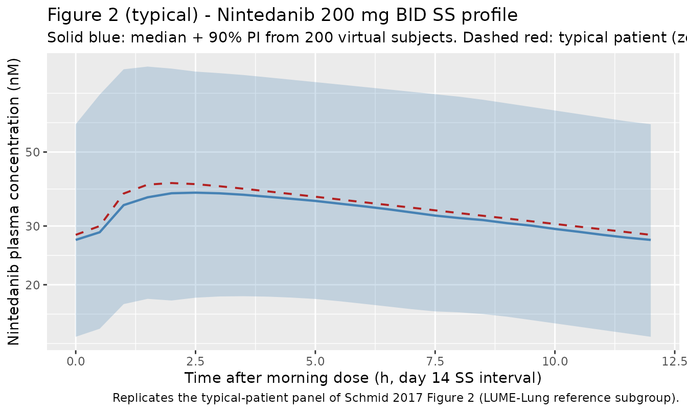
#> ℹ omega/sigma items treated as zero: 'etalfdepot', 'etalka', 'etalvc', 'etalfdepot_bibf'

Replicate published Figure 2 – typical-patient SS profile

Schmid 2017 Figure 2 shows median steady-state nintedanib plasma concentration-time profiles for various covariate subgroups, with the 90% prediction interval of the typical patient as a shaded band. Below we reproduce the typical-patient (Caucasian, age 62, WT 71.5 kg, ex/non-smoker, LUME-Lung 1 reference) curve at 200 mg BID steady state.

ribbon_df <- sim |>
  group_by(time_in_ss) |>
  summarise(
    Q05 = quantile(Cc, 0.05, na.rm = TRUE),
    Q50 = quantile(Cc, 0.50, na.rm = TRUE),
    Q95 = quantile(Cc, 0.95, na.rm = TRUE),
    .groups = "drop"
  )

ggplot(ribbon_df, aes(time_in_ss, Q50)) +
  geom_ribbon(aes(ymin = Q05, ymax = Q95), alpha = 0.25, fill = "steelblue") +
  geom_line(linewidth = 0.8, colour = "steelblue") +
  geom_line(data = sim_typical, aes(time_in_ss, Cc),
            linewidth = 0.7, colour = "firebrick", linetype = "dashed") +
  scale_y_log10() +
  labs(
    x = "Time after morning dose (h, day 14 SS interval)",
    y = "Nintedanib plasma concentration (nM)",
    title = "Figure 2 (typical) - Nintedanib 200 mg BID SS profile",
    subtitle = "Solid blue: median + 90% PI from 200 virtual subjects. Dashed red: typical patient (zeroRe).",
    caption = "Replicates the typical-patient panel of Schmid 2017 Figure 2 (LUME-Lung reference subgroup)."
  )

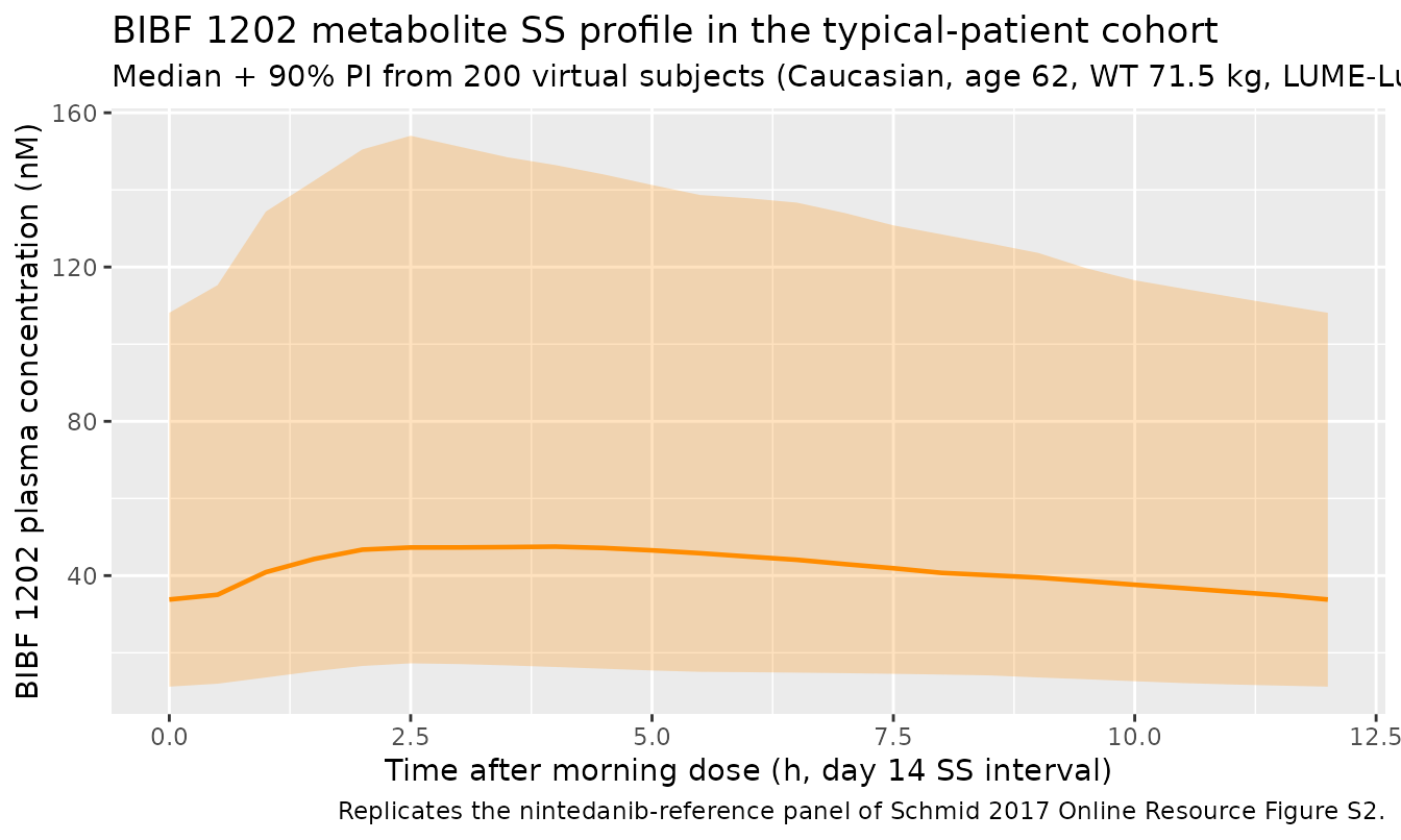
BIBF 1202 metabolite SS profile

The packaged model also returns BIBF 1202 plasma concentrations (Cc_bibf). The typical-patient ratio of BIBF 1202 to nintedanib at steady state should be small (BIBF 1202 is roughly 1% of the F1 dose in first-pass plus a slow systemic-formation flux from ffM = 0.000931).

sim_bibf <- sim |>
  group_by(time_in_ss) |>
  summarise(
    Q05 = quantile(Cc_bibf, 0.05, na.rm = TRUE),
    Q50 = quantile(Cc_bibf, 0.50, na.rm = TRUE),
    Q95 = quantile(Cc_bibf, 0.95, na.rm = TRUE),
    .groups = "drop"
  )

ggplot(sim_bibf, aes(time_in_ss, Q50)) +
  geom_ribbon(aes(ymin = Q05, ymax = Q95), alpha = 0.25, fill = "darkorange") +
  geom_line(linewidth = 0.8, colour = "darkorange") +
  labs(
    x = "Time after morning dose (h, day 14 SS interval)",
    y = "BIBF 1202 plasma concentration (nM)",
    title = "BIBF 1202 metabolite SS profile in the typical-patient cohort",
    subtitle = "Median + 90% PI from 200 virtual subjects (Caucasian, age 62, WT 71.5 kg, LUME-Lung reference).",
    caption = "Replicates the nintedanib-reference panel of Schmid 2017 Online Resource Figure S2."
  )

PKNCA validation (nintedanib at steady state)

PKNCA is used to extract Cmax, Tmax, AUC over the 0-12 h SS interval, and apparent half-life from the simulated profiles, then compared against the expected typical-patient values back-calculated from the published THETA values (Cmax and Tmax not reported in the paper directly; AUCtau,ss = Dose * F1 / (CL/F) = 200 * 1 / 897 = 0.2229 mg/L * h = 222.9 ng/mL * h = 413.1 nM * h).

# Concentrations on the SS interval. Always retain time = 0 (pre-dose at the
# start of the SS interval is the previous dose's 12-h trough; if simulation
# returns NA at that point the bind_rows guard adds an explicit zero).
sim_nca <- sim |>
  filter(!is.na(Cc)) |>
  select(id, time = time_in_ss, Cc, treatment)

# Guarantee a time=0 row per (id, treatment); pre-dose Cc at SS equals the
# previous dose's residual concentration, which the simulation already
# returns at time_in_ss = 0 by construction (the rxSolve grid starts at the
# dose time). The defensive bind_rows ensures the AUC integration is
# anchored even if the simulation grid was reshaped upstream.
sim_nca <- bind_rows(
  sim_nca,
  sim_nca |> distinct(id, treatment) |> mutate(time = 0, Cc = 0)
) |>
  distinct(id, treatment, time, .keep_all = TRUE) |>
  arrange(id, treatment, time)

conc_obj <- PKNCA::PKNCAconc(sim_nca, Cc ~ time | treatment + id)

dose_df <- events |>
  filter(evid == 1L, cmt == "depot") |>
  group_by(id, treatment) |>
  filter(time == max(time[time <= (ss_day - 1) * 24])) |>
  ungroup() |>
  mutate(time = 0) |>  # PKNCA dose time at start of SS interval
  select(id, time, amt, treatment)

dose_obj <- PKNCA::PKNCAdose(dose_df, amt ~ time | treatment + id)

intervals <- data.frame(
  start    = 0,
  end      = 12,
  cmax     = TRUE,
  tmax     = TRUE,
  auclast  = TRUE,
  half.life = TRUE
)

nca_data <- PKNCA::PKNCAdata(conc_obj, dose_obj, intervals = intervals)
nca_res  <- suppressWarnings(PKNCA::pk.nca(nca_data))
nca_summ <- as.data.frame(nca_res$result) |>
  filter(PPTESTCD %in% c("cmax", "tmax", "auclast", "half.life")) |>
  group_by(treatment, PPTESTCD) |>
  summarise(med = stats::median(PPORRES, na.rm = TRUE), .groups = "drop") |>
  pivot_wider(names_from = PPTESTCD, values_from = med)

Typical-patient AUCtau,ss reference

Per Schmid 2017 Table 3 + footer the typical patient (LUME-Lung reference, Caucasian, ex/non-smoker, ECOG >= 1, age 62, WT 71.5 kg) has:

F1 reference = 1
CL/F = 897 L/h
AUCtau,ss = (Dose * F1) / (CL/F) = 200 mg / 897 L/h = 0.2229 mg/L * h = 222.9 ng/mL * h = 413.1 nM * h (using 1 nM = 1.853 ng/mL).

typ_auc_nM_h <- 200 / 897 * 1000 * 1.853  # 200 mg / 897 L/h -> ng/mL * h, then * 1.853 nM per ng/mL
typ_auc_nM_h
#> [1] 413.155

Comparison of the simulated cohort median against the typical-patient reference. The simulated median is the IIV-marginal median, so it reflects the log-normal distribution of CL and F1 in addition to the typical value; the median should land close to (but not identically equal to) the typical-patient value depending on the symmetry of the omega draws.

published <- tibble::tribble(
  ~treatment,                          ~auclast,
  "200 mg BID, LUME-Lung reference",   typ_auc_nM_h
)

cmp <- left_join(nca_summ, published, by = "treatment", suffix = c("_sim", "_pub")) |>
  mutate(pct_diff_auc = 100 * (auclast_sim - auclast_pub) / auclast_pub)

knitr::kable(
  cmp,
  digits = 3,
  caption = "Cohort median NCA at steady state vs the typical-patient reference back-calculated from Schmid 2017 Table 3 (Cmax/Tmax/half-life not published explicitly). The +/- difference vs the typical-patient AUC reflects the asymmetry of the IIV-marginal median around the typical value."
)

Cohort median NCA at steady state vs the typical-patient reference back-calculated from Schmid 2017 Table 3 (Cmax/Tmax/half-life not published explicitly). The +/- difference vs the typical-patient AUC reflects the asymmetry of the IIV-marginal median around the typical value.
treatment	auclast_sim	cmax	half.life	tmax	auclast_pub	pct_diff_auc
200 mg BID, LUME-Lung reference	395.412	38.243	19.44	2	413.155	-4.295

Replicate Table 4 – covariate effects on AUCtau,ss

Schmid 2017 Table 4 reports model-predicted percent changes in nintedanib typical-patient AUCtau,ss for each covariate one at a time, holding all others constant. The block below reproduces a subset of those scenarios by simulating typical-patient profiles (zeroRe) at the same dose, with one covariate flipped to the alternative subgroup, and computing the AUCtau,ss change relative to the LUME-Lung Caucasian reference.

make_typical_events <- function(cov_overrides = list()) {
  c1 <- cohort[1, ]
  for (nm in names(cov_overrides)) c1[[nm]] <- cov_overrides[[nm]]
  bind_rows(
    tibble(id = 1L, time = seq(0, by = dose_int, length.out = n_doses),
           amt = dose_amt, evid = 1L, cmt = "depot"),
    tibble(id = 1L, time = seq(0, by = dose_int, length.out = n_doses),
           amt = dose_amt, evid = 1L, cmt = "depot_bibf"),
    tibble(id = 1L, time = (ss_day - 1) * 24 + obs_times,
           amt = NA_real_, evid = 0L, cmt = "Cc")
  ) |>
    arrange(time, evid) |>
    bind_cols(c1[rep(1L, length.out = NULL), setdiff(names(c1), c("id", "time", "amt", "evid", "cmt"))])
}

cov_simulate <- function(cov_overrides) {
  ev <- make_typical_events(cov_overrides)
  out <- rxode2::rxSolve(mod_typical, events = ev, addCov = TRUE) |> as.data.frame()
  out <- out |> mutate(time_in_ss = time - (ss_day - 1) * 24) |>
    filter(time_in_ss >= 0, time_in_ss <= 12)
  # Trapezoidal AUC over 0-12 h (the SS interval)
  with(out, sum(diff(time_in_ss) * (Cc[-length(Cc)] + Cc[-1]) / 2))
}

# Reference: no overrides
auc_ref <- cov_simulate(list())
#> Warning in rep(1L, length.out = NULL): first element used of 'length.out'
#> argument
#> ℹ omega/sigma items treated as zero: 'etalfdepot', 'etalka', 'etalvc', 'etalfdepot_bibf'

# Scenarios (Schmid 2017 Table 4 row "Nintedanib")
scenarios <- list(
  "Age 45 (5th pctl)"         = list(AGE = 45),
  "Age 76 (95th pctl)"        = list(AGE = 76),
  "Current smoker"            = list(SMOKE = 1L),
  "WT 50 kg (5th pctl)"       = list(WT = 50),
  "WT 100 kg (95th pctl)"     = list(WT = 100),
  "Indian/Chinese/Taiwanese"  = list(RACE_IND_CHI_TWN = 1L, RACE_ASIAN = 1L),
  "Korean"                    = list(RACE_KOREAN = 1L, RACE_ASIAN = 1L)
)

cov_aucs <- vapply(scenarios, cov_simulate, numeric(1))
#> Warning in rep(1L, length.out = NULL): first element used of 'length.out'
#> argument
#> ℹ omega/sigma items treated as zero: 'etalfdepot', 'etalka', 'etalvc', 'etalfdepot_bibf'
#> Warning in rep(1L, length.out = NULL): first element used of 'length.out'
#> argument
#> ℹ omega/sigma items treated as zero: 'etalfdepot', 'etalka', 'etalvc', 'etalfdepot_bibf'
#> Warning in rep(1L, length.out = NULL): first element used of 'length.out'
#> argument
#> ℹ omega/sigma items treated as zero: 'etalfdepot', 'etalka', 'etalvc', 'etalfdepot_bibf'
#> Warning in rep(1L, length.out = NULL): first element used of 'length.out'
#> argument
#> ℹ omega/sigma items treated as zero: 'etalfdepot', 'etalka', 'etalvc', 'etalfdepot_bibf'
#> Warning in rep(1L, length.out = NULL): first element used of 'length.out'
#> argument
#> ℹ omega/sigma items treated as zero: 'etalfdepot', 'etalka', 'etalvc', 'etalfdepot_bibf'
#> Warning in rep(1L, length.out = NULL): first element used of 'length.out'
#> argument
#> ℹ omega/sigma items treated as zero: 'etalfdepot', 'etalka', 'etalvc', 'etalfdepot_bibf'
#> Warning in rep(1L, length.out = NULL): first element used of 'length.out'
#> argument
#> ℹ omega/sigma items treated as zero: 'etalfdepot', 'etalka', 'etalvc', 'etalfdepot_bibf'
cov_table <- tibble(
  Covariate         = names(scenarios),
  Simulated_AUC     = cov_aucs,
  Pct_change        = 100 * (cov_aucs - auc_ref) / auc_ref
) |>
  mutate(
    Published_change_pct = c(
      -16,  # Age 45
      +13,  # Age 76
      -21,  # Current smoker
      +25,  # WT 50
      -19,  # WT 100
      +33,  # Indian/Chinese/Taiwanese
      -22   # Korean
    )
  )

knitr::kable(
  cov_table,
  digits = 2,
  caption = "Schmid 2017 Table 4 reproduction: simulated typical-patient nintedanib AUCtau,ss percent change vs the reference patient (LUME-Lung 1, Caucasian, ex/non-smoker, age 62, WT 71.5 kg) at 200 mg BID steady state."
)

Schmid 2017 Table 4 reproduction: simulated typical-patient nintedanib AUCtau,ss percent change vs the reference patient (LUME-Lung 1, Caucasian, ex/non-smoker, age 62, WT 71.5 kg) at 200 mg BID steady state.
Covariate	Simulated_AUC	Pct_change	Published_change_pct
Age 45 (5th pctl)	345.76	-16.30	-16
Age 76 (95th pctl)	468.57	13.43	13
Current smoker	328.01	-20.60	-21
WT 50 kg (5th pctl)	515.48	24.78	25
WT 100 kg (95th pctl)	335.65	-18.75	-19
Indian/Chinese/Taiwanese	549.43	33.00	33
Korean	322.64	-21.90	-22

If the Pct_change column matches the Published_change_pct column to within 1-2 percentage points for each row, the structural covariate equations and THETA values are reproduced correctly. Any row deviating by more than ~3 percentage points indicates a structural-encoding bug worth investigating (the typical-patient values are deterministic; there is no Monte-Carlo noise in this block).

Assumptions and deviations

IIV in ka uses the Phase II estimate (32.4% CV) only. Schmid 2017 Table 3 reports two separate IIV-in-ka estimates keyed by phase: 32.4% CV from the Phase II studies (NSCLC Phase II and IPF Phase II / TOMORROW, the trials with multiple post-dose samples per subject) and 53.8% CV from the Phase III studies (LUME-Lung 1 and LUME-Lung 2, with sparse sampling). The authors state that the Phase II value is the proper characterization because the Phase III sampling was too sparse to estimate IIV reliably (Table 3 footnote d). The packaged model uses the Phase II value as the single etalka. Users wanting to simulate the Phase III sparse-sampling regime should override etalka to log(1 + 0.538^2) = 0.2511.
Trial-effect covariates encoded as paper-specific composites of canonical STUDY_<id> indicators. Schmid 2017 estimates three trial-effect THETAs that act on F1 (NSCLC Phase II + LUME-Lung 2 vs IPF Phase II + LUME-Lung 1), on ka (NSCLC Phase II + IPF Phase II vs LUME-Lung 1 + LUME-Lung 2), and on BIBF 1202 ka2 (same grouping as nintedanib ka). The dataset carries individual STUDY_TOMORROW, STUDY_NSCLC_NIN_PH2, and STUDY_LUMELUNG2 binaries; the paper’s grouped THETAs are reconstructed inside model() as binary sums of the appropriate pair of indicators. STUDY_LUMELUNG1 is the implicit reference for every trial-effect THETA and is not listed in covariateData because the model body never queries it directly; a LUME-Lung 1 subject is identified as “all four STUDY indicators = 0” in the same way every reference subgroup is identified by the absence of every alternative indicator.
Ethnic-origin covariate uses paper-specific composites that differ between F1 (nintedanib) and F2 (BIBF 1202). For nintedanib F1 the paper groups Indian + Chinese + Taiwanese against a Caucasian / Black / other Asian reference, with Korean as a separate subgroup; this is encoded with the RACE_IND_CHI_TWN composite and the RACE_KOREAN single-subgroup indicator. For BIBF 1202 F2 the paper groups Indian alone (+90%) against Asian-except-Indian (+20%) against a Caucasian / Black reference; this is encoded with the RACE_INDIAN single-subgroup indicator together with a derived race_asian_nonind flag computed in model() as RACE_ASIAN * (1 - RACE_INDIAN). The two new race canonicals (RACE_IND_CHI_TWN, RACE_KOREAN) were ratified by the operator on sidecar 2026-06-21 (request-002, option B); RACE_INDIAN was added in the same extraction as a natural analogue of RACE_KOREAN for the BIBF 1202 Indian-alone effect (the BIBF 1202 covariate was not part of the original Q1 prompt because the supplement containing Table S5 was not yet on disk when sidecar-002 was filed; the supplement was acquired during the current extraction run from https://static-content.springer.com/esm/art%3A10.1007%2Fs00280-017-3452-0/MediaObjects/280_2017_3452_MOESM1_ESM.docx).
ECOG performance status for IPF patients is encoded as ECOG_GE1 = 0. Schmid 2017 Table 2 reports ECOG as “Missing (due to IPF indication) 342 (28.7%)” – the IPF cohort was not scored on the oncology-specific ECOG scale. The source NONMEM model pools these records into the ECOG = 0 reference, which is the convention the packaged model carries forward. A user simulating IPF-only cohorts can use ECOG_GE1 = 0 for all subjects without loss of fidelity vs the paper’s fit.
NSCLC histology for IPF patients is encoded as TUMTP_NSCLC_NONADENO = 0. Schmid 2017 Table 2 pools IPF subjects with “NSCLC of unknown histology” (415 / 1191 subjects = 34.8%) – IPF subjects have no tumour histology. The source model treats these as adenocarcinoma reference for the BIBF 1202 ka2 effect; the packaged model follows the same convention.
units$dosing = "mg" vs units$concentration = "nmol/L" is intentional and dimensionally mismatched. The paper reports doses in mg (mass) and plasma concentrations in nM (molar amount per volume) because the two analytes have closely-similar molecular weights and the molar scale preserves a clean parent/metabolite ratio. The model converts central mass to molar concentration explicitly in model() via the MW-derived conversion factors cf_nint = 1853 (= 1000 ng/mL per mg/L * 1.853 nM per ng/mL, MW nintedanib 539.62 g/mol) and cf_bibf = 1903 (MW BIBF 1202 525.59 g/mol). The convention-check dosing_concentration warning is acknowledged and intentional; downstream simulations should keep doses in mg and read concentrations in nM.
Parameter values come from the SEQUENTIAL fit (Table 3 for nintedanib; Table S5 for BIBF 1202). Schmid 2017 also reports a simultaneous-fit alternative (Online Resource Table S7) where every parameter changes slightly (e.g., theta_CL = 875 vs 897, theta_V2 = 617 vs 465). The sequential fit was reported as the primary final model in the paper’s text and is what we package; the simultaneous fit is a consistency check and could be packaged separately as a sensitivity- analysis variant if a future use case requires it.
ffM (the fraction of nintedanib elimination that produces BIBF 1202 systemically, 0.000931, fixed) was carried over from an upstream healthy- volunteer IV nintedanib study (Schmid 2017 Online Resource Table S4, citing Dallinger et al. 2016 J Clin Pharmacol 56(11):1387-1394 [doi:10.1002/jcph.752]). The current paper used this value as a fixed input to the BIBF 1202 model and did not re-estimate it. Per the skill’s non-paper-provenance rule, the in-file ini() comment for lffm explicitly cites Online Resource Table S4 as the source.
V3/V2 = 0.0185 is fixed from rat IV data (Schmid 2017 ref [14]). The paper notes “the ratio of V3/F-V2/F was fixed based on information observed in rats” without restating the rat-study citation in the main text; the rat data feed into the BIBF 1202 disposition volume. The fixed ratio is encoded via lvc_bibf <- fixed(log(8.6025)) = log(465 * 0.0185).
ALAG2 = ALAG is fixed. Schmid 2017 Online Resource Table S5 reports theta_ALAG2ALAG = 1.00 as fixed. Although the parameter is structurally identifiable, the authors fixed it to the parent ALAG without a substantial change in OFV (DeltaOFV = 1.282) “as besides the comparable estimates of ALAG2 and ALAG, the same absorption delay for both substances was considered plausible”.

Errata

The on-disk PDF is named Schmid_2018_Population_pharmacokinetics_of_nintedani_b579d1.pdf but the paper itself has a 2017 acceptance date and CC-BY 2017 copyright (“Received: 20 June 2017 / Accepted: 10 October 2017 / Published online: 8 November 2017 The Author(s) 2017”). The packaged model file is named Schmid_2017_nintedanib.R per the skill convention (acceptance year) and per the operator’s sidecar-001 decision (response-001 option A, 2026-05-30).
The “Indian / Chinese / Taiwanese” ethnic-origin composite on nintedanib F1 (Schmid 2017 Table 3) and the “Indian alone” composite on BIBF 1202 F2 (Online Resource Table S5) are paper-specific groupings with no obvious biological interpretation; they are empirical clustering results from the covariate-search procedure. They are encoded faithfully here so that any reanalysis can interrogate or refine the groupings – see the canonical register entries RACE_IND_CHI_TWN, RACE_KOREAN, and RACE_INDIAN in inst/references/covariate-columns.md.