Utreloxastat (Hu 2026) • nlmixr2lib

Model and source

#> ℹ parameter labels from comments will be replaced by 'label()'

Citation: Hu Y, Gao L, Kong R. Population Pharmacokinetic Modeling Practice of Time-Varying Clearance: Insights from a First-in-Human Study Case. J Clin Pharmacol. 2026;66(3):e70171. doi:10.1002/jcph.70171
Description: Two-compartment population pharmacokinetic model with an eight-transit- compartment first-order oral absorption chain and time-varying clearance for utreloxastat (PTC857), a 15-lipoxygenase inhibitor in development for amyotrophic lateral sclerosis, in healthy adult volunteers (Hu 2026, the first-in-human study: single ascending doses 100-1000 mg, multiple ascending doses 150-500 mg BID for 14 days, and a three-period food-effect crossover at 500 mg). Apparent clearance fell and the terminal half-life lengthened over repeated dosing (23 h on Day 1 to over 33 h on Day 14), so the authors screened twelve candidate time-varying clearance functions and selected the exponential-in-log-time form (their Model 8), CL(t) = CLTV * (1 + exp(-KTMCL * ln(t))), which is the canonical cl_exp_inf + cl_exp_component * exp(-kdes * .) decomposition with the decaying component’s amplitude equal to CLTV and the decay running against natural-log time after first dose. Absorption is more than dose proportional: relative bioavailability carries a positive power effect of dose level, plus additive increases of 36% for low-fat and 57% for high-fat meals. Age, sex, body weight, BMI, race, ethnicity and hepatic / renal laboratory markers were screened and none was retained.
Article: https://doi.org/10.1002/jcph.70171
Supplement (Tables S1-S3, Figures S1-S3): available from the article’s Supporting Information link.

Hu 2026 is a methods-and-case-study paper. Its scientific contribution is a side-by-side comparison of twelve candidate time-varying-clearance functions fitted to one first-in-human data set, and the model extracted here is the one the authors selected as final: their Model 8, the exponential-in-log-time form, embedded in a two-compartment model with an eight-transit-compartment absorption chain.

Population

68 healthy adult volunteers contributed 1463 quantifiable plasma concentrations from the three parts of a single first-in-human study (Hu 2026 Table 1): 32 participants in the single ascending dose part (100, 250, 500 and 1000 mg, eight per level, taken with a low-fat breakfast), 24 in the multiple ascending dose part (150, 250 and 500 mg twice daily for 14 days with low-fat meals), and 12 in a three-period 500 mg food-effect crossover (fasted, high-fat high-calorie, low-fat low-calorie). Age ranged from 18.0-55.0 years (median 29.5 years) and body weight from 52.4-99.3 kg (median 75.2 kg); 47.1% were female. Race and ethnicity were screened as covariates but their distribution is not tabulated in the paper.

Sampling was intensive to 72 h after dosing in the single-dose and food-effect parts, to 24 h after the Day 1 dose and to 72 h after the Day 14 morning dose in the multiple-dose part, with a single additional pre-dose sample on Day 7 (supplemental Table S3). That near-absence of data between Day 1 and Day 14 is the reason the authors give for the curvature of the clearance-versus-time function being only weakly identified.

The same information is available programmatically via rxode2::rxode(readModelDb("Hu_2026_utreloxastat"))$population.

Source trace

Every ini() entry in inst/modeldb/specificDrugs/Hu_2026_utreloxastat.R carries an in-file comment naming its source location. They are collected here for review.

Equation / parameter	Value	Source location
`lktr` (paper `Ka`)	4.10 1/h	Table 3 theta1; the Table 3 footnote uses the same number as the chain’s “transit constant” in MTT = (8 + 1) / 4.10 = 2.20 h
`lvc` (paper `V/F`)	362.00 L	Table 3 theta2
`lcl_exp_inf` (paper `CL/F`, `CL_TV`)	46.85 L/h	Table 3 theta3
`lvp` (paper `V2/F`)	1827.15 L	Table 3 theta4
`lq` (paper `Q/F`)	37.39 L/h	Table 3 theta5
`expSd` (paper “Additive residual”)	0.46	Table 3 theta6; Methods observation equation `Ln(Y) = Ln(f(theta, eta, t)) + epsilon`
`e_fed_lowfat_fdepot`	0.36	Table 3 theta7
`e_fed_highfat_fdepot`	0.57	Table 3 theta8
`e_dose_fdepot`	0.21	Table 3 theta9
`lcl_exp_kdes` (paper `KTMCL`)	0.096	Table 3 theta10; supplemental Table S1, Model 8 row
`etalktr`	0.16 (variance)	Table 3 ETA/IIV row 1 (IIV-Ka, %CV 42.26, shrinkage 1.21%)
`etalcl_exp_inf`	0.027 (variance)	Table 3 ETA/IIV row 2 (IIV-CL/F, %CV 16.53, shrinkage 11.24%)
Number of transit compartments (8)	n/a	Results, “Model Structure and Pharmacokinetic Parameters”; Table 3 footnote; supplemental Figure S3
`CL_TV,t = CL_TV * (1 + exp(-KTMCL * ln(t)))`	n/a	Table 2, Model 8
`Frel` additive meal terms, power dose term	n/a	Methods (“a power model was used for continuous covariates, and a binominal model was used for categorical covariates”); Table 3 theta7-theta9
Two-compartment disposition	n/a	Results, “Model Structure and Pharmacokinetic Parameters”
Reference dose 250 mg in the `Frel` power term	250 mg	Not printed by the paper. Adopted from Table 5 / Figure 4 (“Reference: 250 mg/BID/fasted”) and the Table 1 SAD and MAD median dose. See Assumptions and deviations.

Reading the two variance-versus-SD choices off the reported precision

Table 3 gives an estimate and an asymptotic standard error for the residual and for each IIV term but does not say which scale each is on. Both are settled by the Cramer-Rao lower bound, which caps how precisely a variance or a standard deviation can possibly be estimated from a given number of observations.

n_obs  <- 1463  # quantifiable PK observations (Hu 2026 Results, "Demographics")
n_subj <- 68    # participants

# Residual: Table 3 reports estimate 0.46, ASE 0.0091.
crlb_var_resid <- 0.46 * sqrt(2 / n_obs)   # lower bound on SE if 0.46 were a variance
crlb_sd_resid  <- 0.46 / sqrt(2 * n_obs)   # lower bound on SE if 0.46 were an SD
c(reported_ase = 0.0091, bound_if_variance = crlb_var_resid, bound_if_sd = crlb_sd_resid)
#>      reported_ase bound_if_variance       bound_if_sd 
#>       0.009100000       0.017007899       0.008503949

An ASE of 0.0091 is below the bound that a variance estimate could achieve (0.017) and above the bound for a standard-deviation estimate (0.0085), so 0.46 is a standard deviation. The IIV terms go the other way:

# IIV-CL/F: Table 3 reports estimate 0.027, ASE 0.0059, "%CV" 16.53.
c(reported_ase       = 0.0059,
  bound_if_variance  = 0.027 * sqrt(2 / n_subj),
  cv_if_variance_pct = 100 * sqrt(exp(0.027) - 1),
  cv_if_sd_pct       = 100 * sqrt(exp(0.027^2) - 1))
#>       reported_ase  bound_if_variance cv_if_variance_pct       cv_if_sd_pct 
#>        0.005900000        0.004630462       16.543216968        2.700492150

Reading 0.027 as a log-scale variance reproduces the printed 16.53% coefficient of variation through sqrt(exp(omega^2) - 1); reading it as a standard deviation would give about 2.7%. The model file therefore encodes etalcl_exp_inf ~ 0.027 and etalktr ~ 0.16 as variances and expSd <- 0.46 as a standard deviation.

stopifnot(
  0.0091 < 0.46 * sqrt(2 / n_obs),         # 0.46 cannot be a variance
  0.0091 > 0.46 / sqrt(2 * n_obs),         # it is feasible as an SD
  abs(100 * sqrt(exp(0.027) - 1) - 16.53) < 0.1  # matches the printed %CV
)

The time-varying clearance function

Table 2 of Hu 2026 lists twelve candidate functions. Model 8, the one carried into the final model, is

$CL_{TV,t} = CL_{TV}\,\bigl(1 + e^{-K_{TMCL}\ln t}\bigr) = CL_{TV}\,\bigl(1 + t^{-K_{TMCL}}\bigr)$

with $CL_{TV}$ = 46.85 L/h and $K_{TMCL}$ = 0.096. It is a member of the cl_exp_ family registered in the package conventions (cl_exp_inf + cl_exp_component * exp(-cl_exp_kdes * .)), distinguished from its siblings by having no separate fractional amplitude (so the decaying component’s amplitude equals $CL_{TV}$ itself) and by running the decay against $\ln t$ rather than $t$ .

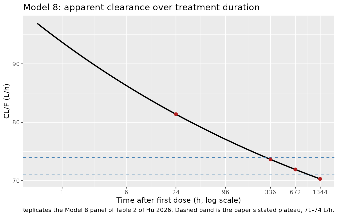
The paper reports one quantitative anchor for the whole family: across all twelve candidate models the apparent clearance “consistently showed similar values at the plateau stage, approximately 71 to 74 L/h” (the blue dashed line in Table 2). That is the check below.

cl_tv <- function(t, cl = 46.85, ktmcl = 0.096) cl * (1 + exp(-ktmcl * log(t)))

cl_grid <- tibble(time = 10^seq(log10(0.5), log10(24 * 56), length.out = 400)) |>
  mutate(cl = cl_tv(time))

anchors <- tibble(
  label = c("Day 1 (24 h)", "Day 14 (336 h)", "4 weeks (672 h)", "8 weeks (1344 h)"),
  time  = c(24, 336, 672, 1344)
) |>
  mutate(cl = cl_tv(time))

knitr::kable(
  anchors |> dplyr::rename("Time point" = label, "Time (h)" = time, "CL/F (L/h)" = cl),
  digits = 1,
  caption = "Apparent clearance from Model 8 at four time points."
)

Apparent clearance from Model 8 at four time points.
Time point	Time (h)	CL/F (L/h)
Day 1 (24 h)	24	81.4
Day 14 (336 h)	336	73.7
4 weeks (672 h)	672	71.9
8 weeks (1344 h)	1344	70.3

# Hu 2026 Results: the plateau of the clearance-vs-time curve is ~71-74 L/h,
# and the Discussion places the plateau "after 4 weeks".
cl_4wk <- cl_tv(672)
stopifnot(
  cl_4wk >= 71 && cl_4wk <= 74,
  cl_tv(336) >= 71 && cl_tv(336) <= 74,
  # The curve is still monotone decreasing but has flattened: less than 3%
  # further change over the fortnight following the stated plateau time.
  cl_tv(672) < cl_tv(336),
  abs(cl_tv(1344) / cl_tv(672) - 1) < 0.03
)
cl_4wk
#> [1] 71.92738

# Replicates the Model 8 panel of Table 2 of Hu 2026: apparent clearance
# declining over treatment duration towards a plateau.
ggplot(cl_grid, aes(time, cl)) +
  geom_line(linewidth = 0.9) +
  geom_hline(yintercept = c(71, 74), linetype = "dashed", colour = "steelblue") +
  geom_point(data = anchors, colour = "firebrick", size = 2) +
  scale_x_log10(breaks = c(1, 6, 24, 96, 336, 672, 1344)) +
  labs(
    x = "Time after first dose (h, log scale)", y = "CL/F (L/h)",
    title = "Model 8: apparent clearance over treatment duration",
    caption = paste(
      "Replicates the Model 8 panel of Table 2 of Hu 2026.",
      "Dashed band is the paper's stated plateau, 71-74 L/h."
    )
  )

The ln(t) singularity and the numerical floor

Hu 2026 flags a limitation of its own selected model in the Discussion: “applying a natural logarithm transformation of predose time (time = 0) results in undefined values (approaching infinity)”. The paper does not say how the fit handled it, so the model file floors the time argument at 0.01 h.

The claim made for that floor is that it is numerically inert, not a modelling choice: at 0.01 h the dose has barely started to leave depot and still has eight transit compartments to cross, so essentially nothing is in central while the floor is active. The check below re-solves the model with the floor moved over four orders of magnitude and compares the resulting profiles.

mod <- readModelDb("Hu_2026_utreloxastat")

single_dose_events <- function(dose, lowfat = 1, highfat = 0, id = 1L,
                               times = c(seq(0, 12, by = 0.1), seq(12.5, 72, by = 0.5))) {
  ev <- dplyr::bind_rows(
    tibble(id = id, time = 0, amt = dose, evid = 1L, cmt = "depot"),
    tibble(id = id, time = times, amt = NA_real_, evid = 0L, cmt = "central")
  )
  ev |>
    mutate(
      DOSE_UTRELOXASTAT_MG = dose,
      FED_LOWFAT           = lowfat,
      FED_HIGHFAT          = highfat
    ) |>
    arrange(time, desc(evid))
}

# `rxode2::model()` replaces the one line of the model body that sets the
# floor. Three literal calls rather than a function of the floor value, so
# the substituted number is visible in the source.
mod_floor_lo  <- rxode2::model(mod, tcl <- max(time, 0.0001), auto = FALSE)
#> ℹ parameter labels from comments will be replaced by 'label()'
mod_floor_mid <- mod                                    # the packaged 0.01 h
mod_floor_hi  <- rxode2::model(mod, tcl <- max(time, 0.5), auto = FALSE)
#> ℹ parameter labels from comments will be replaced by 'label()'

ev_floor <- single_dose_events(500)
solve_floor <- function(m) {
  rxode2::rxSolve(rxode2::zeroRe(m), ev_floor, returnType = "data.frame",
                  useLinCmt = FALSE) |>
    dplyr::filter(time > 0) |>
    dplyr::pull(Cc)
}
cc_lo  <- solve_floor(mod_floor_lo)
#> ℹ omega/sigma items treated as zero: 'etalktr', 'etalcl_exp_inf'
cc_mid <- solve_floor(mod_floor_mid)
#> ℹ parameter labels from comments will be replaced by 'label()'
#> ℹ omega/sigma items treated as zero: 'etalktr', 'etalcl_exp_inf'
cc_hi  <- solve_floor(mod_floor_hi)
#> ℹ omega/sigma items treated as zero: 'etalktr', 'etalcl_exp_inf'
stopifnot(length(cc_lo) == length(cc_mid), length(cc_hi) == length(cc_mid),
          length(cc_mid) > 100, all(cc_mid > 0))

max_rel_diff <- max(abs(cc_lo / cc_mid - 1), abs(cc_hi / cc_mid - 1))
max_rel_diff
#> [1] 0.0003036787

# The floor must not be doing any work: moving it from 0.0001 h to 0.5 h --
# a factor of 5000 -- may not change any predicted concentration by more than
# 0.1%. If this ever fails, the floor has become a modelling assumption and
# must be re-derived from the source rather than kept for convenience.
stopifnot(max_rel_diff < 1e-3)

Virtual cohort

Original observed data are not publicly available. Two cohorts are used below. The first is a deterministic (zeroRe) typical-value cohort with one subject per arm, used wherever the target is a published typical-value quantity or an exposure ratio: with the random effects zeroed, additional subjects would be exact duplicates. The second is a stochastic cohort of 50 subjects per dose arm, used for the concentration-time figures.

set.seed(20260829)

# Dose levels of the single-ascending-dose part (Hu 2026 Table 1). All SAD
# doses were taken with a low-fat breakfast (Methods, "PK Data Collection").
sad_doses <- c(100, 250, 500, 1000)

sad_typical <- dplyr::bind_rows(
  lapply(seq_along(sad_doses), function(i) {
    single_dose_events(sad_doses[i], id = i) |>
      mutate(treatment = paste0(sad_doses[i], " mg"))
  })
)
stopifnot(!anyDuplicated(unique(sad_typical[, c("id", "time", "evid")])))

# Stochastic cohort: 50 subjects per dose arm, IDs offset so they are disjoint,
# observed at the study's ACTUAL Day 1 single-dose sampling times (supplemental
# Table S3). Sampling on the protocol grid rather than a dense grid is what
# makes the Tmax comparison below apples-to-apples: an NCA Tmax can only ever
# land on a scheduled time, so a model whose true peak is at 3.1 h is recorded
# as 3 h or 4 h depending on the subject.
protocol_times <- c(0.5, 1, 2, 3, 4, 6, 8, 10, 12, 24, 48, 72)

n_per_arm <- 50L
sad_stochastic <- dplyr::bind_rows(
  lapply(seq_along(sad_doses), function(i) {
    dplyr::bind_rows(lapply(seq_len(n_per_arm), function(j) {
      single_dose_events(
        sad_doses[i],
        id    = (i - 1L) * n_per_arm + j,
        times = c(0, protocol_times)
      )
    })) |>
      mutate(treatment = paste0(sad_doses[i], " mg"))
  })
)
stopifnot(!anyDuplicated(unique(sad_stochastic[, c("id", "time", "evid")])))
nrow(sad_stochastic)
#> [1] 2800

The multiple-dose arms follow the study design: twice-daily dosing for 14 days, so the Day 14 morning dose is the 27th dose, at 312 h. Observations cover the Day 1 interval and the Day 14 interval plus its 72 h tail.

mad_events <- function(dose, lowfat = 1, highfat = 0, id = 1L, tail = TRUE,
                       n_doses = 27L) {
  dose_times <- seq(0, by = 12, length.out = n_doses)
  obs_times <- c(seq(0, 24, by = 0.25), seq(312, 324, by = 0.1))
  if (tail) obs_times <- c(obs_times, seq(324.5, 384, by = 1))
  ev <- dplyr::bind_rows(
    tibble(id = id, time = dose_times, amt = dose, evid = 1L, cmt = "depot"),
    tibble(id = id, time = sort(unique(obs_times)), amt = NA_real_,
           evid = 0L, cmt = "central")
  )
  ev |>
    mutate(
      DOSE_UTRELOXASTAT_MG = dose,
      FED_LOWFAT           = lowfat,
      FED_HIGHFAT          = highfat
    ) |>
    arrange(time, desc(evid))
}

# Five typical-value arms reproducing the covariate scenarios of Table 5:
# the 250 mg BID fasted reference, the 5th and 95th dose percentiles, and the
# two meal conditions at the reference dose.
forest_arms <- tibble::tribble(
  ~treatment,        ~dose, ~lowfat, ~highfat,
  "250 mg (ref)",     250,        0,        0,
  "150 mg",           150,        0,        0,
  "500 mg",           500,        0,        0,
  "Low-fat meal",     250,        1,        0,
  "High-fat meal",    250,        0,        1
)

forest_events <- dplyr::bind_rows(
  lapply(seq_len(nrow(forest_arms)), function(i) {
    mad_events(forest_arms$dose[i], forest_arms$lowfat[i], forest_arms$highfat[i],
               id = i, tail = FALSE) |>
      mutate(treatment = forest_arms$treatment[i])
  })
)
stopifnot(!anyDuplicated(unique(forest_events[, c("id", "time", "evid")])))

Simulation

useLinCmt = FALSE is passed to every solve. rxode2’s automatic ODE-to-linCmt() conversion assumes a time-invariant elimination rate; this model’s kel changes with time, so the conversion must be suppressed.

mod_typical <- rxode2::zeroRe(mod)
#> ℹ parameter labels from comments will be replaced by 'label()'

sim_sad_typical <- rxode2::rxSolve(
  mod_typical, sad_typical, keep = "treatment",
  returnType = "data.frame", useLinCmt = FALSE
)
#> ℹ omega/sigma items treated as zero: 'etalktr', 'etalcl_exp_inf'
#> Warning: multi-subject simulation without without 'omega'

sim_sad <- rxode2::rxSolve(
  mod, sad_stochastic, keep = "treatment",
  returnType = "data.frame", useLinCmt = FALSE
)
#> ℹ parameter labels from comments will be replaced by 'label()'

sim_forest <- rxode2::rxSolve(
  mod_typical, forest_events, keep = "treatment",
  returnType = "data.frame", useLinCmt = FALSE
)
#> ℹ omega/sigma items treated as zero: 'etalktr', 'etalcl_exp_inf'
#> Warning: multi-subject simulation without without 'omega'

A first structural check: the clearance the solver actually used must equal the Model 8 function evaluated at the same time.

stopifnot("cl" %in% names(sim_sad_typical))
cl_check <- sim_sad_typical |>
  filter(time > 1) |>
  mutate(cl_expected = cl_tv(time))
stopifnot(nrow(cl_check) > 100,
          max(abs(cl_check$cl / cl_check$cl_expected - 1)) < 1e-8)

Replicate published figures

Figure 1: dose-normalized single-dose profiles

Figure 1 of Hu 2026 plots dose-normalized concentrations after single ascending doses and makes one qualitative point: the curves do not superimpose, and higher doses sit above lower ones, which the paper reads as more-than-dose- proportional absorption. The terminal phases are nonetheless parallel on the log scale, which the paper reads as elimination that is not saturable.

dose_lookup <- tibble(treatment = paste0(sad_doses, " mg"), dose = sad_doses)

vpc_bands <- sim_sad |>
  filter(time > 0) |>
  group_by(treatment, time) |>
  summarise(
    Q05 = quantile(Cc, 0.05), Q50 = median(Cc), Q95 = quantile(Cc, 0.95),
    .groups = "drop"
  ) |>
  left_join(dose_lookup, by = "treatment") |>
  mutate(across(c(Q05, Q50, Q95), ~ .x / dose))

typical_curves <- sim_sad_typical |>
  filter(time > 0) |>
  left_join(dose_lookup, by = "treatment") |>
  mutate(cc_dn = Cc / dose)

ggplot(vpc_bands, aes(time, Q50, colour = treatment, fill = treatment)) +
  geom_ribbon(aes(ymin = Q05, ymax = Q95), alpha = 0.15, colour = NA) +
  geom_line(data = typical_curves, aes(time, cc_dn, colour = treatment),
            inherit.aes = FALSE, linewidth = 0.8) +
  geom_point(size = 1.4) +
  scale_y_log10() +
  labs(
    x = "Time after dose (h)", y = "Dose-normalized Cc (ng/mL per mg)",
    colour = "Dose", fill = "Dose",
    title = "Dose-normalized single-dose profiles",
    caption = paste(
      "Replicates Figure 1b of Hu 2026. Lines are typical-value profiles;",
      "points and ribbons are the median and 5th-95th percentile of 50",
      "simulated subjects per arm at the study's Table S3 sampling times."
    )
  )

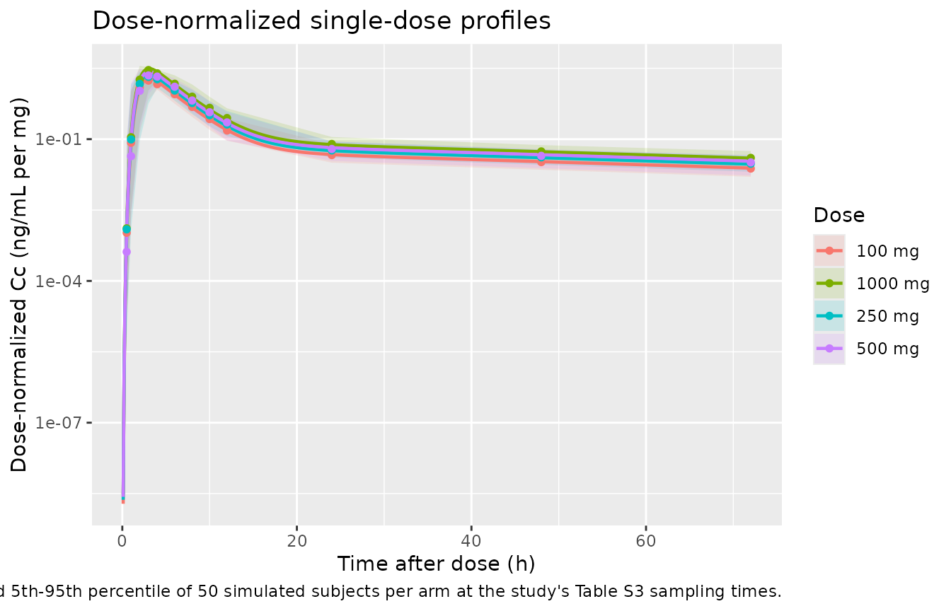
# The paper's two readings of Figure 1, as assertions on typical-value curves.
dn <- sim_sad_typical |>
  filter(time > 0) |>
  left_join(tibble(treatment = paste0(sad_doses, " mg"), dose = sad_doses),
            by = "treatment") |>
  mutate(cc_dn = Cc / dose)

peak_dn <- dn |> group_by(dose) |> summarise(peak = max(cc_dn), .groups = "drop") |>
  arrange(dose)

# (1) Dose-normalized peak concentration increases monotonically with dose.
stopifnot(all(diff(peak_dn$peak) > 0))
# (2) The dose effect is entirely on F, so every arm shares one profile shape
#     and the 1000 mg / 100 mg dose-normalized peak ratio is exactly 10^0.21.
stopifnot(abs(peak_dn$peak[4] / peak_dn$peak[1] - 10^0.21) < 1e-8)
# (3) Terminal slopes are parallel: elimination is not concentration-dependent,
#     so every dose level shares one terminal slope exactly.
term_slope <- dn |>
  filter(time >= 48, time <= 72) |>
  group_by(dose) |>
  summarise(slope = coef(lm(log(cc_dn) ~ time))[2], .groups = "drop")
stopifnot(diff(range(term_slope$slope)) < 1e-8)
peak_dn
#> # A tibble: 4 × 2
#>    dose  peak
#>   <dbl> <dbl>
#> 1   100  1.91
#> 2   250  2.32
#> 3   500  2.68
#> 4  1000  3.10

Figure 2c: Day 1 versus Day 14

Figure 2c compares the Day 1 and Day 14 profiles of the multiple-dose part and reports “a lower elimination rate than Day1 across all dose levels after the morning dose”. Hu 2026 quantifies this in the Introduction from the companion non-compartmental analysis: a terminal half-life of 23 h on Day 1 rising to over 33 h on Day 14.

mad_tail <- rxode2::rxSolve(
  mod_typical, mad_events(250, id = 1L),
  returnType = "data.frame", useLinCmt = FALSE
)
#> ℹ omega/sigma items treated as zero: 'etalktr', 'etalcl_exp_inf'

profiles <- dplyr::bind_rows(
  mad_tail |> filter(time > 0, time <= 24) |>
    transmute(tad = time, Cc, day = "Day 1"),
  mad_tail |> filter(time >= 312) |>
    transmute(tad = time - 312, Cc, day = "Day 14")
)

ggplot(profiles, aes(tad, Cc, colour = day)) +
  geom_line(linewidth = 0.9) +
  scale_y_log10() +
  labs(
    x = "Time after morning dose (h)", y = "Cc (ng/mL)", colour = NULL,
    title = "250 mg BID: Day 1 versus Day 14",
    caption = "Replicates Figure 2c of Hu 2026 (typical-value profiles)."
  )

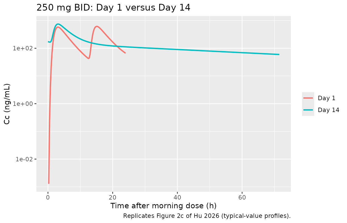
The apparent half-life this model produces depends strongly on the window it is measured over, so the window has to be stated before the comparison means anything. The Day 1 curve below is the 500 mg single-dose arm, because the Day 1 profile of the BID cohort is interrupted by the evening dose; the two arms share every disposition parameter.

half_life_over <- function(df, lo, hi) {
  d <- df |> filter(tad >= lo, tad <= hi, Cc > 0)
  stopifnot(nrow(d) >= 3)
  log(2) / -coef(lm(log(Cc) ~ tad, data = d))[[2]]
}
sad_500 <- sim_sad_typical |> filter(treatment == "500 mg", time > 0) |>
  transmute(tad = time, Cc)
day14 <- profiles |> filter(day == "Day 14")

windows <- tibble::tribble(
  ~lo, ~hi,
    8,  24,
   10,  24,
   12,  24,
   24,  48,
   24,  72
) |>
  mutate(
    window = sprintf("%.0f-%.0f h", lo, hi),
    day1   = mapply(half_life_over, list(sad_500), lo, hi),
    day14  = mapply(half_life_over, list(day14), lo, hi),
    ratio  = day14 / day1
  )

windows |>
  dplyr::select(window, day1, day14, ratio) |>
  dplyr::rename(
    "Fitting window"     = window,
    "Day 1 t1/2 (h)"     = day1,
    "Day 14 t1/2 (h)"    = day14,
    "Day 14 / Day 1"     = ratio
  ) |>
  knitr::kable(digits = 2,
               caption = "Apparent half-life by lambda-z fitting window.")

Apparent half-life by lambda-z fitting window.
Fitting window	Day 1 t1/2 (h)	Day 14 t1/2 (h)	Day 14 / Day 1
8-24 h	4.52	10.87	2.40
10-24 h	5.30	13.78	2.60
12-24 h	7.34	19.13	2.61
24-48 h	50.28	51.66	1.03
24-72 h	52.26	52.30	1.00

The model’s true terminal half-life is the one the 24-72 h window recovers, and it can be computed exactly from the micro-constants rather than by regression:

terminal_half_life <- function(t, vc = 362, vp = 1827.15, q = 37.39) {
  kel <- cl_tv(t) / vc
  k12 <- q / vc
  k21 <- q / vp
  s <- kel + k12 + k21
  beta <- 0.5 * (s - sqrt(s^2 - 4 * kel * k21))
  log(2) / beta
}
c(day1 = terminal_half_life(48), day14 = terminal_half_life(360))
#>     day1    day14 
#> 50.93351 52.31278

# What the paper claims, and the model supports, is DIRECTIONAL: the apparent
# terminal phase is flatter on Day 14 than on Day 1.
stopifnot(
  all(windows$ratio > 1),                                       # every window
  windows$ratio[windows$window == "12-24 h"] > 2,               # and strongly so
  terminal_half_life(360) > terminal_half_life(48)              # exactly, too
)

The comparison against the paper’s absolute numbers needs care, and the disagreement is reported rather than tuned away. Hu 2026’s Introduction quotes 23 h on Day 1 and over 33 h on Day 14 from the companion non-compartmental publication (its reference 16), which is not in this repository, so the window those lambda-z values were fitted over is unknown. The design constrains it: in the multiple-dose cohort, Day 1 was sampled only to 24 h post dose while Day 14 was sampled to 72 h (supplemental Table S3), so the two published half-lives cannot have come from the same window. Over the intermediate windows a 24-hour Day 1 profile allows, the model reproduces both the direction and roughly the magnitude of the reported lengthening (12-24 h: 7.3 h to 19.1 h). Over the full 24-72 h window it converges on its true terminal half-life of about 52 h on both days, which is more than double the published Day 1 value.

That is a genuine feature of the parameterisation, not a transcription error. The terminal eigenvalue of this model is dominated by return from the large peripheral compartment, k21 = Q/F / (V2/F) = 0.0205 1/h, which Model 8 leaves time-invariant. A 24% fall in clearance between Day 1 and Day 14 therefore moves the terminal half-life by only about 2.7%, even though it moves exposure substantially. All four disposition parameters were re-checked against Table 3 before this note was written.

PKNCA validation

Single dose

sim_nca <- sim_sad |>
  dplyr::filter(!is.na(Cc)) |>
  dplyr::select(id, time, Cc, treatment)

# Guarantee a time = 0 row per (id, treatment); pre-dose Cc = 0 for an
# extravascular dose.
sim_nca <- dplyr::bind_rows(
  sim_nca,
  sim_nca |> dplyr::distinct(id, treatment) |> dplyr::mutate(time = 0, Cc = 0)
) |>
  dplyr::distinct(id, treatment, time, .keep_all = TRUE) |>
  dplyr::arrange(id, treatment, time)

conc_obj <- PKNCA::PKNCAconc(sim_nca, Cc ~ time | treatment + id)

dose_df <- sad_stochastic |>
  dplyr::filter(evid == 1) |>
  dplyr::select(id, time, amt, treatment)
dose_obj <- PKNCA::PKNCAdose(dose_df, amt ~ time | treatment + id)

intervals <- data.frame(
  start = 0, end = 72,
  cmax = TRUE, tmax = TRUE, auclast = TRUE, half.life = TRUE
)

nca_res <- PKNCA::pk.nca(PKNCA::PKNCAdata(conc_obj, dose_obj, intervals = intervals))

nca_wide <- as.data.frame(nca_res) |>
  dplyr::filter(PPTESTCD %in% c("cmax", "tmax", "auclast", "half.life")) |>
  dplyr::group_by(treatment, PPTESTCD) |>
  dplyr::summarise(value = median(PPORRES), .groups = "drop") |>
  tidyr::pivot_wider(names_from = PPTESTCD, values_from = value)

nca_wide |>
  dplyr::relocate(treatment, cmax, tmax, auclast, half.life) |>
  dplyr::rename(
    "Dose"                 = treatment,
    "Cmax (ng/mL)"         = cmax,
    "Tmax (h)"             = tmax,
    "AUC0-72 (h*ng/mL)"    = auclast,
    "t1/2 (h)"             = half.life
  ) |>
  knitr::kable(digits = c(0, 1, 2, 0, 1),
               caption = "Median simulated single-dose NCA by dose level.")

Median simulated single-dose NCA by dose level.
Dose	Cmax (ng/mL)	Tmax (h)	AUC0-72 (h*ng/mL)	t1/2 (h)
100 mg	184.3	3.0	1139	50.0
1000 mg	2988.8	3.0	18795	50.0
250 mg	578.4	3.0	3508	50.1
500 mg	1261.6	3.5	7805	49.5

Comparison against published NCA

Hu 2026 reports no absolute simulated or observed exposure values of its own; Table 4 gives only percentages within the prediction interval and prediction-to-observation ratios, and Table 5 gives only exposure ratios. The two absolute single-dose descriptors it does quote, from the companion non-compartmental publication (Hu 2026 Introduction, citing reference 16), are a Tmax of 4 h and a Day 1 terminal half-life of 23 h. Both are pooled single-dose descriptors rather than per-dose-level values, so the same reference number is repeated for each arm below.

published <- tibble::tibble(
  treatment = paste0(sad_doses, " mg"),
  tmax      = 4,
  half.life = 23
)

cmp <- nlmixr2lib::ncaComparisonTable(
  simulated     = nca_res,
  reference     = published,
  by            = "treatment",
  units         = c(tmax = "h", half.life = "h"),
  tolerance_pct = 20
)

knitr::kable(
  cmp,
  caption = paste(
    "Simulated vs. published single-dose NCA.",
    "* differs from the reference by more than 20%."
  )
)

Simulated vs. published single-dose NCA. * differs from the reference by more than 20%.
NCA parameter	treatment	Reference	Simulated	% diff
Tmax (h)	100 mg	4	3	-25.0%*
Tmax (h)	250 mg	4	3	-25.0%*
Tmax (h)	500 mg	4	3.5	-12.5%
Tmax (h)	1000 mg	4	3	-25.0%*
t½ (h)	100 mg	23	50	+117.4%*
t½ (h)	250 mg	23	50.1	+118.0%*
t½ (h)	500 mg	23	49.5	+115.2%*
t½ (h)	1000 mg	23	50	+117.6%*

Both rows are starred, and they are starred for different reasons. Neither was tuned towards.

Tmax: 3 h simulated against 4 h published. In relative terms that is -25%, which trips the 20% flag, but in absolute terms it is one sampling interval: the protocol grid runs 3, 4, 6 h through the peak, so 3 h and 4 h are adjacent scheduled times and no intermediate value is observable. The model’s underlying peak is at 3.1 h, a direct structural consequence of the transit chain (eight transit compartments at 4.10 1/h, mean transit time 2.20 h). This is the sense in which the flag overstates the disagreement: percent difference is a poor metric for a parameter whose resolution is set by a coarse and unevenly spaced design grid.

Half-life: about 50 h simulated against 23 h published. This one is a real disagreement in magnitude, for the window reason analysed in the preceding section, and it is not an artefact of the metric.

med <- function(code) {
  v <- as.data.frame(nca_res) |>
    dplyr::filter(PPTESTCD == code) |>
    dplyr::pull(PPORRES) |>
    stats::median()
  if (!is.finite(v)) stop("no finite median for ", code)
  v
}
tmax_typical <- typical_curves$time[which.max(typical_curves$cc_dn)]

stopifnot(
  # Deterministic: the typical-value peak is within one protocol sampling
  # interval of the 4 h the paper reports.
  abs(tmax_typical - 4) <= 1,
  # Stochastic median lands on a scheduled sampling time next to it.
  med("tmax") %in% c(3, 4),
  # The comparison table did produce a starred row, i.e. the >20% flag is
  # really being raised rather than silently absent.
  any(vapply(cmp, function(x) any(grepl("*", as.character(x), fixed = TRUE)),
             logical(1)))
)
c(tmax_typical = tmax_typical, tmax_median = med("tmax"),
  half_life_median = med("half.life"))
#>     tmax_typical      tmax_median half_life_median 
#>          3.10000          3.00000         49.98658

Steady-state exposure ratios (Table 5)

Table 5 of Hu 2026 reports the covariate forest-plot output: steady-state Cmax, Cmin and AUC0-12 h after the morning dose of a BID regimen, each as a ratio to a 250 mg BID fasted reference. Because clearance in this model depends on time but not on concentration, the system is linear in dose amount, so these ratios are exactly reproducible from typical-value profiles.

ss_nca <- sim_forest |>
  dplyr::filter(!is.na(Cc)) |>
  dplyr::select(id, time, Cc, treatment)

ss_conc <- PKNCA::PKNCAconc(ss_nca, Cc ~ time | treatment + id)
ss_dose <- PKNCA::PKNCAdose(
  forest_events |> dplyr::filter(evid == 1) |>
    dplyr::select(id, time, amt, treatment),
  amt ~ time | treatment + id
)

ss_intervals <- data.frame(
  start = 312, end = 324,
  cmax = TRUE, cmin = TRUE, auclast = TRUE
)
ss_res <- PKNCA::pk.nca(PKNCA::PKNCAdata(ss_conc, ss_dose, intervals = ss_intervals))

ss_wide <- as.data.frame(ss_res) |>
  dplyr::filter(PPTESTCD %in% c("cmax", "cmin", "auclast")) |>
  dplyr::select(treatment, PPTESTCD, PPORRES) |>
  tidyr::pivot_wider(names_from = PPTESTCD, values_from = PPORRES)

ref_row <- ss_wide |> dplyr::filter(treatment == "250 mg (ref)")
ratios <- ss_wide |>
  dplyr::mutate(
    cmax_ratio = cmax / ref_row$cmax,
    cmin_ratio = cmin / ref_row$cmin,
    auc_ratio  = auclast / ref_row$auclast
  ) |>
  dplyr::select(treatment, cmax_ratio, cmin_ratio, auc_ratio)

published_t5 <- tibble::tribble(
  ~treatment,       ~cmax_pub, ~cmin_pub, ~auc_pub,
  "250 mg (ref)",        1.00,      1.00,     1.00,
  "150 mg",              0.54,      0.53,     0.53,
  "500 mg",              2.30,      2.26,     2.28,
  "Low-fat meal",        1.36,      1.36,     1.37,
  "High-fat meal",       1.56,      1.56,     1.56
)

t5 <- ratios |>
  dplyr::left_join(published_t5, by = "treatment") |>
  dplyr::relocate(treatment, cmax_ratio, cmax_pub, cmin_ratio, cmin_pub,
                  auc_ratio, auc_pub)

t5 |>
  dplyr::rename(
    "Scenario"           = treatment,
    "Cmax,ss (sim)"      = cmax_ratio,
    "Cmax,ss (Table 5)"  = cmax_pub,
    "Cmin,ss (sim)"      = cmin_ratio,
    "Cmin,ss (Table 5)"  = cmin_pub,
    "AUC0-12,ss (sim)"   = auc_ratio,
    "AUC0-12,ss (Table 5)" = auc_pub
  ) |>
  knitr::kable(
    digits = 2,
    caption = paste(
      "Steady-state exposure ratios relative to 250 mg BID fasted.",
      "Simulated values are typical-value; Table 5 values are medians of",
      "1000 parametric-bootstrap replicates."
    )
  )

Steady-state exposure ratios relative to 250 mg BID fasted. Simulated values are typical-value; Table 5 values are medians of 1000 parametric-bootstrap replicates.
Scenario	Cmax,ss (sim)	Cmax,ss (Table 5)	Cmin,ss (sim)	Cmin,ss (Table 5)	AUC0-12,ss (sim)	AUC0-12,ss (Table 5)
150 mg	0.54	0.54	0.54	0.53	0.54	0.53
250 mg (ref)	1.00	1.00	1.00	1.00	1.00	1.00
500 mg	2.31	2.30	2.31	2.26	2.31	2.28
High-fat meal	1.57	1.56	1.57	1.56	1.57	1.56
Low-fat meal	1.36	1.36	1.36	1.36	1.36	1.37

stopifnot(nrow(t5) == 5L, !anyNA(t5))
# Every simulated ratio must land within 5% of the published one. The
# residual gap is the Monte-Carlo noise of the paper's 1000-replicate
# bootstrap plus its two-decimal rounding, not a structural disagreement:
# the model's dose ratios are exactly (dose/250)^1.21 and its meal ratios
# exactly 1.36 and 1.57.
worst <- max(abs(c(
  t5$cmax_ratio / t5$cmax_pub,
  t5$cmin_ratio / t5$cmin_pub,
  t5$auc_ratio  / t5$auc_pub
) - 1))
stopifnot(worst < 0.03)

# The closed forms, asserted exactly.
stopifnot(
  abs(t5$auc_ratio[t5$treatment == "150 mg"]        - (150 / 250)^1.21) < 1e-3,
  abs(t5$auc_ratio[t5$treatment == "500 mg"]        - (500 / 250)^1.21) < 1e-3,
  abs(t5$auc_ratio[t5$treatment == "Low-fat meal"]  - 1.36) < 1e-3,
  abs(t5$auc_ratio[t5$treatment == "High-fat meal"] - 1.57) < 1e-3
)
worst
#> [1] 0.02361778

The exponent 1.21 is the sum of the dose itself (exponent 1) and the bioavailability power term (exponent 0.21), which is why exposure rises slightly faster than the dose.

Accumulation ratio (Table 4)

Table 4 of Hu 2026 gives model-predicted AUC0-12 h accumulation ratios of 1.4 to 1.8 across dose levels, against observed ratios of 1.3 to 2.2. The dose-to-dose spread of the predicted values is a regimen artefact rather than a dose effect: the table’s footnote records that the 150 mg and 250 mg cohorts stepped down to once-daily dosing part way through, while the 500 mg cohort stayed on BID throughout. Only the 500 mg regimen is unambiguous, and because the model is linear in dose the ratio for a clean BID regimen is the same at any dose level.

acc_int <- data.frame(
  start = c(0, 312), end = c(12, 324), auclast = TRUE
)
# Subset to the reference arm first; the only filter applied to the
# concentration frame itself is `!is.na(Cc)`, so the time = 0 record that
# anchors AUC0-12 h survives.
acc_arm <- sim_forest[sim_forest$treatment == "250 mg (ref)", ]
acc_conc <- PKNCA::PKNCAconc(
  acc_arm |> dplyr::filter(!is.na(Cc)) |> dplyr::select(id, time, Cc),
  Cc ~ time | id
)
acc_dose_rows <- forest_events[forest_events$treatment == "250 mg (ref)", ]
acc_dose <- PKNCA::PKNCAdose(
  acc_dose_rows |> dplyr::filter(evid == 1) |> dplyr::select(id, time, amt),
  amt ~ time | id
)
stopifnot(any(acc_arm$time == 0))
acc_res <- as.data.frame(
  PKNCA::pk.nca(PKNCA::PKNCAdata(acc_conc, acc_dose, intervals = acc_int))
) |>
  dplyr::filter(PPTESTCD == "auclast")

acc_ratio <- acc_res$PPORRES[acc_res$start == 312] /
  acc_res$PPORRES[acc_res$start == 0]
acc_ratio
#> [1] 1.697138

# Hu 2026 Table 4: predicted AUC0-12 h accumulation ratios span 1.4 to 1.8
# across dose levels, observed 1.3 to 2.2.
stopifnot(acc_ratio > 1, acc_ratio >= 1.4, acc_ratio <= 1.8)

Accumulation here is greater than a time-invariant model fitted to Day 1 would predict, because clearance falls from about 86.3 L/h during the first dosing interval to about 73.8 L/h by Day 14. That is the effect the paper set out to characterise, and it is why the paper warns that the accumulation-based effective-half-life calculation of the earlier non-compartmental analysis is no longer valid: that calculation assumes a constant clearance and a steady state that this model says has not been reached by Day 14.

Assumptions and deviations

Reference dose in the bioavailability power term (250 mg). Hu 2026 states the power form for continuous covariates and reports the exponent (Table 3 theta9 = 0.21) but never prints the dose the term is normalized to. 250 mg is adopted here because it is the reference of the paper’s own covariate forest plot (Figure 4 and Table 5, “Reference: 250 mg/BID/fasted”) and the median dose of both the SAD and MAD cohorts (Table 1). The constant cancels out of every exposure ratio the paper publishes, so no reported number can falsify it; it does set the absolute concentration scale, which the paper never reports in absolute units either. A user who prefers a different normalization should change the 250 in f(depot) and rescale lcl_exp_inf, lvc, lvp and lq accordingly, since all four are apparent (per unit bioavailability) parameters.
ln(t) floor at 0.01 h. The selected Model 8 is undefined at t = 0, a limitation the paper states but does not resolve. The floor is verified above to be numerically inert over four orders of magnitude, so it is a solver guard rather than a modelling assumption.
t is time after first dose, not time after the most recent dose. Table 2 of Hu 2026 spells TAD explicitly where it means time after dose (Model 4 only); Models 5 through 12, including the selected Model 8, use t, and the paper describes it in the Methods observation equation as “longitudinal Time”. The Model 8 panel in Table 2, whose x-axis runs out to four weeks and whose plateau the paper places “after 4 weeks”, is only interpretable on that reading.
Residual error is lnorm, not proportional. The Methods observation equation is additive on the natural-log scale, which is nlmixr2’s lnorm(). For a residual standard deviation of 0.46 the two are not interchangeable: lnorm gives a median-unbiased multiplicative error, whereas a proportional model at that magnitude admits negative concentrations.
Variance-versus-SD scales. Hu 2026 does not label the scale of its Table 3 uncertainty column. The residual is encoded as a standard deviation and both IIVs as log-scale variances, each settled against the Cramer-Rao bound and the printed %CV column as shown in the Source trace section.
The high-fat meal effect is stated inconsistently by the paper; 0.57 is used. Table 3 (theta8) and the Results section both give 57%, with a 90% confidence interval of 42% to 72%. The Discussion’s closing summary instead reads “72% (90% CI: 42% to 72%) for high-fat meals”, repeating the interval’s upper bound in place of the point estimate. The paper adjudicates itself: its Table 5 forest-plot output gives a steady-state AUC ratio of 1.56 for high-fat versus fasted, matching 1 + 0.57 = 1.57 and excluding 1 + 0.72 = 1.72. The check is made explicitly in the Steady-state exposure ratios section above, where the simulated high-fat ratio is asserted against 1.57. No erratum for this article was located.
Meal-condition pooling. FED_LOWFAT = 1 covers three protocol conditions that the paper pooled: the food-effect part’s low-fat low-calorie meal, the site-standardized meal used throughout the SAD and MAD parts, and a customized medium-fat meal that was not statistically distinguishable from low-fat. This makes FED_LOWFAT = 1 the usual state in this study rather than a special arm, and it means the fasted reference (FED_LOWFAT = 0, FED_HIGHFAT = 0) is informed only by one period of the 12-subject food-effect crossover.
Screened but unused covariates. Age, sex, body weight, BMI, race, ethnicity, albumin, ALP, ALT, AST, total bilirubin and creatinine were all screened and none was retained; no point estimates are published for them. They are recorded in the model file’s covariatesDataExcluded metadata so the provenance of the covariate screen is preserved without declaring covariates the model never uses.
Eleven of the twelve Table 2 candidate functions are not extracted. The package convention is to extract the model the authors selected as final. Table 2 and supplemental Table S1 are a model-selection exercise, and the eleven rejected candidates are reported with explicit reasons for rejection (unacceptable estimates, failed covariance steps, or clearance falling by 100% within 24 h); most of them are not reported with a complete parameter set, so they could not be reconstructed even if wanted.
The published terminal half-life is not reproduced, and was not tuned towards. Hu 2026 quotes 23 h on Day 1 and over 33 h on Day 14 from its companion non-compartmental publication. Fitted over the full 24-72 h window this model gives about 52 h on both days; fitted over the shorter windows the Day 1 design actually permits, it gives roughly the reported values and the reported lengthening. The section Figure 2c works this through. The disagreement is a property of the published parameter set – the terminal eigenvalue is dominated by the time-invariant Q/F / (V2/F) return rate – and the four disposition parameters were re-verified against Table 3 rather than adjusted.
Tmax is 3.1 h, against the 4 h the paper quotes. On the Table S3 grid that is one sampling interval, but it is a 25% relative difference and is therefore starred in the comparison table above. Also not tuned.
No absolute exposure target exists in the source. Every quantitative validation above is therefore a ratio, a time, or a clearance value. The absolute concentration scale of this model rests on the reference-dose choice documented in the first bullet.