Fosfomycin intravenous and oral (Ortiz Zacarias 2018)
Source:vignettes/articles/OrtizZacarias_2018_fosfomycin.Rmd
OrtizZacarias_2018_fosfomycin.RmdModel and source
iv <- rxode2::rxode(readModelDb("OrtizZacarias_2018_fosfomycin_iv"))
#> ℹ parameter labels from comments will be replaced by 'label()'
po <- rxode2::rxode(readModelDb("OrtizZacarias_2018_fosfomycin_oral"))
#> ℹ parameter labels from comments will be replaced by 'label()'- Citation: Ortiz Zacarias NV, Dijkmans AC, Burggraaf J, Mouton JW, Wilms EB, van Nieuwkoop C, Touw DJ, Kamerling IMC, Stevens J. Fosfomycin as a potential therapy for the treatment of systemic infections: a population pharmacokinetic model to simulate multiple dosing regimens. Pharmacol Res Perspect. 2018;6(1):e00378. doi:10.1002/prp2.378
- Article: https://doi.org/10.1002/prp2.378
- Intravenous model:
OrtizZacarias_2018_fosfomycin_iv - Oral model:
OrtizZacarias_2018_fosfomycin_oral
This paper is unusual and the shape of the extraction follows from that. Ortiz Zacarias 2018 fitted no data of its own. It is a simulation study: the authors assembled a structural model and a complete parameter set out of two previously published analyses, resampled the reported parameter uncertainty and inter-individual variability to build 1000 virtual subjects, and used the result to ask whether any oral fosfomycin regimen can reach serum concentrations adequate for a systemic infection. Every number in the two model files is therefore a transcription of a transcription, and the paper’s own Tables 2 and 3 are the answer key against which this vignette checks the transcription.
Why two model files
Section 2.1 describes two structures, not one:
“The structural model for intravenous administration was based on a previously reported two-compartment population PK model of fosfomycin, developed on 12 patients scheduled for abscess drainage. […] To include oral administration of fosfomycin tromethamine, the model was extended with a gastrointestinal- (GI) and a transit component (TRANS) […] Additionally, a transfer constant representing biliary clearance of the drug (kb) was included in the oral PK model.”
Figure 1 draws both overlaid, so it is easy to read it as a single
model in which kb always drains the central compartment. It
is not, and the paper’s own tables settle it: carrying kb
into the intravenous model would add
kb * Vc = 0.50 * 10.1 = 5.05 L/h of elimination on top of
CL = 5.808 L/h and cut the Table 2 intravenous AUC roughly
in half (see “Assumptions and deviations” for the arithmetic). Table 2
is reproduced only without kb, and Table 3 only with it.
The two structures are therefore packaged as two files, per the
library’s replicate-the-author’s-structure policy, with this single
vignette covering the paper as a unit.
Structure and symbol map
Figure 1 numbers its compartments; the model files use the library’s canonical role-based names. The mapping is:
| Figure 1 | Canonical name | Role |
|---|---|---|
| CMT 1 “GI” | depot |
oral dosing compartment (gut) |
| CMT 2 “TRANS” | transit1 |
transit compartment |
| CMT 3 “Central” | central |
central, volume Vc
|
| CMT 4 “Peripheral” | peripheral1 |
peripheral, volume Vp
|
k12 (CMT 1 -> 2) |
ka |
absorptive route out of the gut depot |
k10 (out of CMT 1) |
kfec |
competing loss of unabsorbed drug; sets bioavailability |
k23 (CMT 2 -> 3) |
ktr |
transit compartment into central |
kb (out of CMT 3) |
kbile |
apparent biliary elimination (oral model only) |
Q |
q |
intercompartmental clearance |
CL |
cl |
clearance |
k56, k61 (grey) |
not implemented | enterohepatic recirculation, excluded by the authors |
Enterohepatic recirculation (Figure 1, grey: CMT 5 biliary tract
-> CMT 6 transit -> CMT 1 GI) was tested and rejected in Section
3.1 (“it was decided to exclude this PK property from the model”), so
k56 and k61 are deliberately absent and
kbile is a terminal elimination route rather than a
recycling one.
cat(rxode2::modelExtract(po, endpoint = TRUE), sep = "\n")
#> Cc ~ add(addSd)
Population
str(po$population)
#> List of 9
#>  $ species       : chr "human"
#>  $ n_subjects    : int 17
#>  $ n_studies     : int 2
#>  $ age_range     : chr "Adults; not further specified by Ortiz Zacarias 2018"
#>  $ disease_state : chr "Two upstream cohorts pooled at the parameter level rather than at the data level: 12 patients scheduled for abs"| __truncated__
#>  $ dose_range    : chr "Simulated oral regimens of fosfomycin tromethamine: 2-15 g per dose every 8 h, and 3 and 6 g every 12 or 24 h ("| __truncated__
#>  $ regions       : chr "Not reported"
#>  $ renal_function: chr "Simulated CLCR mean 103 mL/min, SD 41 mL/min, truncated between the minimum and maximum values reported by Saue"| __truncated__
#>  $ notes         : chr "Ortiz Zacarias 2018 fitted NO data of its own. It is a simulation study: the structural model and every paramet"| __truncated__
No subject was studied by Ortiz Zacarias 2018. The parameters rest on
two upstream cohorts pooled at the parameter level: 12 patients
scheduled for abscess drainage (Kjellsson et al., reference 25 of the
source paper; source of CL, Vc,
Vp, Q and their variability) and 5 healthy
volunteers dosed orally and intravenously (Segre et al., reference 24;
source of k10, k12, k23 and
kb). The creatinine-clearance distribution used to drive
the covariate model comes from a third published cohort
(Sauermann et al., reference 32): mean 103 mL/min, SD 41 mL/min,
truncated at that paper’s reported minimum and maximum.
Source trace
Every ini() value carries an in-file comment naming its
origin. Collected here:
| Equation / parameter | Value | Source location |
|---|---|---|
lcl (CL) |
5.808 L/h (90% CI 3.792-7.80) | Table 1, row CL (Kjellsson et al.) |
lvc (Vc) |
10.1 L (90% CI 5.36-14.8) | Table 1, row Vc |
lvp (Vp) |
9.80 L (90% CI 5.70-13.9) | Table 1, row Vp |
lq (Q) |
15.36 L/h (90% CI 9.12-21.6) | Table 1, row Q |
lka (paper k12) |
1.69 1/h (SD 0.62) | Table 1, row k12 (Segre et al.) |
lkfec (paper k10) |
1.24 1/h (SD 0.55) | Table 1, row k10 |
lktr (paper k23) |
0.34 1/h (SD 0.10) | Table 1, row k23 |
lkbile (paper kb) |
0.50 1/h (SD 0.18) | Table 1, row kb |
e_crcl_cl |
0.0141 L/h per mL/min | Table 1, row COV CLCR-CL; Equation 5 |
| CLCR centering value | 103 mL/min | Equation 5; Section 2.2 (from Sauermann et al.) |
etalcl |
0.238 (variance) | Table 1, CL row, IIV column |
etalvc |
0.238 * 1.64 = 0.39032 (variance) | Table 1, Vc row, IIV column (printed literally as
0.238 * 1.64) |
etalvp |
0.197 (variance) | Table 1, Vp row, IIV column |
no eta on q
|
“NI” (not identified) | Table 1, Q row, IIV column |
| no eta on the four rate constants | “ND” (no data available) | Table 1, IIV column |
addSd |
fixed(0) |
no residual-error model is reported anywhere in the paper |
theta_i = theta_TV * exp(eta_i) |
n/a | Equation 1 |
CL_i = [CL_TV + 0.0141 * (CLCR_i - 103)] * exp(eta_i) |
n/a | Equation 5 |
| compartment structure and connectivity | n/a | Figure 1 (black portion) |
The IIV column holds variances, not SDs or CVs. Section 2.1 states it explicitly: “eta is assumed to be normally distributed around 0 with its reported variance omega^2.”
The parameter-uncertainty layer
Equations 2 to 4 describe a layer that sits above the model: before drawing a subject’s etas, the authors draw that subject’s typical value from an uncertainty distribution derived from the published 90% CI or SD. In the log domain,
- Equation 3:
omega2_LN = log(sigma2_N / theta2_p,N + 1) - Equation 2:
theta_p,LN = log(theta_p,N) - omega2_LN / 2
This is a simulation protocol, not model structure, so it is not part
of ini(). But Table 1’s “Uncertainty (variance)” column is
itself a derived quantity – footnote a says “Calculated from the 90% CI
or SD” – which makes it a check on the transcription of the intervals. A
90% CI of a normal spans 2 * qnorm(0.95) = 3.2897 SDs.
unc <- tibble::tribble(
  ~Parameter, ~mean,  ~lo,    ~hi,   ~sd,   ~printed,
  "CL",        5.808,  3.792,  7.80,  NA,     1.4841,
  "Vc",       10.1,    5.36,  14.8,   NA,     8.2329,
  "Vp",        9.80,   5.70,  13.9,   NA,     6.2120,
  "Q",        15.36,   9.12,  21.6,   NA,    14.3892,
  "k10",       1.24,  NA,     NA,     0.55,   0.3025,
  "k12",       1.69,  NA,     NA,     0.62,   0.3844,
  "k23",       0.34,  NA,     NA,     0.10,   0.0100,
  "kb",        0.50,  NA,     NA,     0.18,   0.0324
) |>
  dplyr::mutate(
    derived = dplyr::if_else(
      is.na(sd),
      ((hi - lo) / (2 * stats::qnorm(0.95)))^2,
      sd^2
    ),
    pct_diff = 100 * (derived - printed) / printed
  )

unc |>
  dplyr::select(Parameter, printed, derived, pct_diff) |>
  dplyr::rename(
    "Table 1 uncertainty variance" = printed,
    "Recomputed from CI / SD" = derived,
    "% diff" = pct_diff
  ) |>
knitr::kable(digits = c(0, 4, 4, 3))| Parameter | Table 1 uncertainty variance | Recomputed from CI / SD | % diff |
|---|---|---|---|
| CL | 1.4841 | 1.4844 | 0.018 |
| Vc | 8.2329 | 8.2344 | 0.018 |
| Vp | 6.2120 | 6.2132 | 0.019 |
| Q | 14.3892 | 14.3918 | 0.018 |
| k10 | 0.3025 | 0.3025 | 0.000 |
| k12 | 0.3844 | 0.3844 | 0.000 |
| k23 | 0.0100 | 0.0100 | 0.000 |
| kb | 0.0324 | 0.0324 | 0.000 |
# Deterministic arithmetic, so a tight bound is the right bound: this can only
# go red if a mean, an interval bound or a standard deviation was mis-read.
stopifnot(max(abs(unc$pct_diff)) < 0.2)
All eight rows reproduce, the four SD-derived ones exactly and the four CI-derived ones to better than 0.03%. The transcription of Table 1 is sound.
The log-domain uncertainty variances that follow from Equation 3 are
what a user would pass to rxode2::rxSolve(thetaMat = ) to
add this layer back:
logVar <- function(variance, mean) log(variance / mean^2 + 1)
thetaMat <- diag(c(
  lcl = logVar(1.4841, 5.808),
  lvc = logVar(8.2329, 10.1),
  lvp = logVar(6.2120, 9.80),
  lq  = logVar(14.3892, 15.36)
))
dimnames(thetaMat) <- list(
  c("lcl", "lvc", "lvp", "lq"),
  c("lcl", "lvc", "lvp", "lq")
)
round(diag(thetaMat), 5)
#>     lcl     lvc     lvp      lq
#> 0.04306 0.07762 0.06268 0.05920
Derived bioavailability
The gut depot drains by two competing first-order routes, so the
fraction of an oral dose that reaches the transit compartment is
ka / (ka + kfec). The paper never prints this number, but
it is what its k10 exists to produce:
ka <- exp(po$theta[["lka"]])
kfec <- exp(po$theta[["lkfec"]])
c(ka = ka, kfec = kfec, F_oral = ka / (ka + kfec))
#>        ka      kfec    F_oral
#> 1.6900000 1.2400000 0.5767918
About 58% of an oral dose is absorbed. Note that this is not
the apparent oral bioavailability one would infer from the AUC ratio
between Table 3 and Table 2, because the oral model also carries the
extra kbile elimination route.
Typical-value reproduction of the published tables
The strongest check available is the paper’s own output. Both tables
report steady-state exposure over a 24 h window (“AUC/MIC was calculated
over a period of 24 hours at steady state”, Section 2.5), so that is
what is computed here, from a typical-value (zeroRe) solve
at the covariate reference CRCL = 103.
# One typical-value steady-state profile, re-based so the window starts at 0.
# `addl` must carry dosing THROUGH the end of the 24 h window, not merely up to
# its start, or the window silently loses its last dose.
ssProfile <- function(mod, doseMg, ii, cmt, tinf = NA_real_, grid = 0.005) {
  nCycle <- 11L + ceiling(24 / ii)
  ev <-
    if (is.na(tinf)) {
      rxode2::et(amt = doseMg, cmt = cmt, ii = ii, addl = nCycle)
    } else {
      rxode2::et(amt = doseMg, cmt = cmt, ii = ii, addl = nCycle, rate = doseMg / tinf)
    }
  t0 <- 11 * ii
  ev <- rxode2::et(ev, seq(t0, t0 + 24, by = grid))
  out <-
    rxode2::rxSolve(
      rxode2::zeroRe(mod),
      events = ev,
      params = c(CRCL = 103),
      returnType = "data.frame",
      atol = 1e-12, rtol = 1e-12
    )
  out <- out[out$time >= t0, c("time", "Cc")]
  out$time <- out$time - t0
  out
}

trapz <- function(d) sum(diff(d$time) * (utils::head(d$Cc, -1) + utils::tail(d$Cc, -1)) / 2)

# Fraction of ONE dosing interval spent above the MIC.
pctTgtMIC <- function(d, ii, mic = 8) {
  w <- d[d$time <= ii, ]
  mid <- (utils::head(w$Cc, -1) + utils::tail(w$Cc, -1)) / 2
  100 * sum(diff(w$time)[mid > mic]) / ii
}
Oral regimens against Table 3
Table 3’s med column is the median of the paper’s
1000-subject simulation; because the oral model is linear in dose and
the only covariate sits at its reference value here, the typical-value
profile is the right comparator.
oralRef <- tibble::tribble(
  ~dose_g, ~ii, ~cmax,  ~auc,     ~pct_t_mic,
  2,        8,   18.96,  316.95,   84,
  3,        8,   28.44,  475.42,  100,
  3,       12,   24.52,  313.48,   66,
  3,       24,   22.87,  154.26,   31,
  4,        8,   37.93,  633.89,  100,
  5,        8,   47.41,  792.36,  100,
  6,        8,   56.89,  950.84,  100,
  6,       12,   47.70,  602.87,   87,
  6,       24,   44.12,  296.83,   42,
  7,        8,   66.37, 1109.31,  100,
  8,        8,   75.85, 1267.78,  100,
  9,        8,   85.33, 1426.26,  100,
 10,        8,   94.81, 1584.73,  100,
 11,        8,  104.30, 1743.20,  100,
 12,        8,  113.78, 1901.67,  100,
 15,        8,  142.22, 2377.09,  100
) |>
  dplyr::mutate(treatment = sprintf("%g g q%gh", dose_g, ii))

oralSim <- do.call(
  rbind,
  lapply(seq_len(nrow(oralRef)), function(i) {
    p <- ssProfile(po, oralRef$dose_g[i] * 1000, oralRef$ii[i], "depot")
    data.frame(
      treatment = oralRef$treatment[i],
      cmax = max(p$Cc),
      auclast = trapz(p),
      pct_t_mic = pctTgtMIC(p, oralRef$ii[i])
    )
  })
)
#> ℹ omega/sigma items treated as zero: 'etalcl', 'etalvc', 'etalvp'
#> ℹ omega/sigma items treated as zero: 'etalcl', 'etalvc', 'etalvp'
#> ℹ omega/sigma items treated as zero: 'etalcl', 'etalvc', 'etalvp'
#> ℹ omega/sigma items treated as zero: 'etalcl', 'etalvc', 'etalvp'
#> ℹ omega/sigma items treated as zero: 'etalcl', 'etalvc', 'etalvp'
#> ℹ omega/sigma items treated as zero: 'etalcl', 'etalvc', 'etalvp'
#> ℹ omega/sigma items treated as zero: 'etalcl', 'etalvc', 'etalvp'
#> ℹ omega/sigma items treated as zero: 'etalcl', 'etalvc', 'etalvp'
#> ℹ omega/sigma items treated as zero: 'etalcl', 'etalvc', 'etalvp'
#> ℹ omega/sigma items treated as zero: 'etalcl', 'etalvc', 'etalvp'
#> ℹ omega/sigma items treated as zero: 'etalcl', 'etalvc', 'etalvp'
#> ℹ omega/sigma items treated as zero: 'etalcl', 'etalvc', 'etalvp'
#> ℹ omega/sigma items treated as zero: 'etalcl', 'etalvc', 'etalvp'
#> ℹ omega/sigma items treated as zero: 'etalcl', 'etalvc', 'etalvp'
#> ℹ omega/sigma items treated as zero: 'etalcl', 'etalvc', 'etalvp'
#> ℹ omega/sigma items treated as zero: 'etalcl', 'etalvc', 'etalvp'
# PKNCA on the same typical-value steady-state windows. The input filter is
# !is.na(Cc) ONLY -- a `time > 0` or `Cc > 0` filter would drop the t = 0 record
# and trigger PKNCA's "AUC range starting before the first measurement" warning
# once per profile.
oralConcRaw <- do.call(
  rbind,
  lapply(seq_len(nrow(oralRef)), function(i) {
    p <- ssProfile(po, oralRef$dose_g[i] * 1000, oralRef$ii[i], "depot", grid = 0.02)
    data.frame(treatment = oralRef$treatment[i], time = p$time, Cc = p$Cc)
  })
) |>
  dplyr::filter(!is.na(Cc))
#> ℹ omega/sigma items treated as zero: 'etalcl', 'etalvc', 'etalvp'
#> ℹ omega/sigma items treated as zero: 'etalcl', 'etalvc', 'etalvp'
#> ℹ omega/sigma items treated as zero: 'etalcl', 'etalvc', 'etalvp'
#> ℹ omega/sigma items treated as zero: 'etalcl', 'etalvc', 'etalvp'
#> ℹ omega/sigma items treated as zero: 'etalcl', 'etalvc', 'etalvp'
#> ℹ omega/sigma items treated as zero: 'etalcl', 'etalvc', 'etalvp'
#> ℹ omega/sigma items treated as zero: 'etalcl', 'etalvc', 'etalvp'
#> ℹ omega/sigma items treated as zero: 'etalcl', 'etalvc', 'etalvp'
#> ℹ omega/sigma items treated as zero: 'etalcl', 'etalvc', 'etalvp'
#> ℹ omega/sigma items treated as zero: 'etalcl', 'etalvc', 'etalvp'
#> ℹ omega/sigma items treated as zero: 'etalcl', 'etalvc', 'etalvp'
#> ℹ omega/sigma items treated as zero: 'etalcl', 'etalvc', 'etalvp'
#> ℹ omega/sigma items treated as zero: 'etalcl', 'etalvc', 'etalvp'
#> ℹ omega/sigma items treated as zero: 'etalcl', 'etalvc', 'etalvp'
#> ℹ omega/sigma items treated as zero: 'etalcl', 'etalvc', 'etalvp'
#> ℹ omega/sigma items treated as zero: 'etalcl', 'etalvc', 'etalvp'

oralDose <- do.call(
  rbind,
  lapply(seq_len(nrow(oralRef)), function(i) {
    data.frame(
      treatment = oralRef$treatment[i],
      time = seq(0, 24 - oralRef$ii[i], by = oralRef$ii[i]),
      dose = oralRef$dose_g[i] * 1000
    )
  })
)

oralNca <-
  PKNCA::pk.nca(
    PKNCA::PKNCAdata(
      PKNCA::PKNCAconc(oralConcRaw, Cc ~ time | treatment),
      PKNCA::PKNCAdose(oralDose, dose ~ time | treatment),
      intervals = data.frame(start = 0, end = 24, cmax = TRUE, auclast = TRUE)
    )
  )

oralCmp <-
  nlmixr2lib::ncaComparisonTable(
    simulated = as.data.frame(oralNca),
    reference =
      oralRef |>
        dplyr::select(treatment, cmax, auclast = auc),
    by = "treatment",
    units = c(cmax = "mg/L", auclast = "mg/L*h")
  )
knitr::kable(oralCmp)| NCA parameter | treatment | Reference | Simulated | % diff |
|---|---|---|---|---|
| Cmax (mg/L) | 2 g q8h | 19 | 18.9 | -0.1% |
| Cmax (mg/L) | 3 g q8h | 28.4 | 28.4 | -0.1% |
| Cmax (mg/L) | 3 g q12h | 24.5 | 24.8 | +1.3% |
| Cmax (mg/L) | 3 g q24h | 22.9 | 23.5 | +2.9% |
| Cmax (mg/L) | 4 g q8h | 37.9 | 37.9 | -0.1% |
| Cmax (mg/L) | 5 g q8h | 47.4 | 47.4 | -0.1% |
| Cmax (mg/L) | 6 g q8h | 56.9 | 56.8 | -0.1% |
| Cmax (mg/L) | 6 g q12h | 47.7 | 49.7 | +4.1% |
| Cmax (mg/L) | 6 g q24h | 44.1 | 47.1 | +6.7% |
| Cmax (mg/L) | 7 g q8h | 66.4 | 66.3 | -0.1% |
| Cmax (mg/L) | 8 g q8h | 75.8 | 75.8 | -0.1% |
| Cmax (mg/L) | 9 g q8h | 85.3 | 85.3 | -0.1% |
| Cmax (mg/L) | 10 g q8h | 94.8 | 94.7 | -0.1% |
| Cmax (mg/L) | 11 g q8h | 104 | 104 | -0.1% |
| Cmax (mg/L) | 12 g q8h | 114 | 114 | -0.1% |
| Cmax (mg/L) | 15 g q8h | 142 | 142 | -0.1% |
| AUClast (mg/L*h) | 2 g q8h | 317 | 319 | +0.6% |
| AUClast (mg/L*h) | 3 g q8h | 475 | 478 | +0.6% |
| AUClast (mg/L*h) | 3 g q12h | 313 | 319 | +1.7% |
| AUClast (mg/L*h) | 3 g q24h | 154 | 159 | +3.3% |
| AUClast (mg/L*h) | 4 g q8h | 634 | 637 | +0.6% |
| AUClast (mg/L*h) | 5 g q8h | 792 | 797 | +0.6% |
| AUClast (mg/L*h) | 6 g q8h | 951 | 956 | +0.6% |
| AUClast (mg/L*h) | 6 g q12h | 603 | 637 | +5.7% |
| AUClast (mg/L*h) | 6 g q24h | 297 | 319 | +7.4% |
| AUClast (mg/L*h) | 7 g q8h | 1110 | 1120 | +0.6% |
| AUClast (mg/L*h) | 8 g q8h | 1270 | 1270 | +0.6% |
| AUClast (mg/L*h) | 9 g q8h | 1430 | 1430 | +0.6% |
| AUClast (mg/L*h) | 10 g q8h | 1580 | 1590 | +0.6% |
| AUClast (mg/L*h) | 11 g q8h | 1740 | 1750 | +0.6% |
| AUClast (mg/L*h) | 12 g q8h | 1900 | 1910 | +0.6% |
| AUClast (mg/L*h) | 15 g q8h | 2380 | 2390 | +0.6% |
attr(oralCmp, "footnote")
#> NULL
oralChk <- dplyr::inner_join(oralRef, oralSim, by = "treatment", suffix = c("_ref", "_sim"))
oralChk <- dplyr::mutate(
  oralChk,
  cmax_pct = 100 * (cmax_sim - cmax_ref) / cmax_ref,
  auc_pct = 100 * (auclast - auc) / auc,
  tmic_diff = pct_t_mic_sim - pct_t_mic_ref
)

# Deterministic typical-value solves -- no cohort is drawn, so these bounds do
# not depend on rxode2's thread-partitioned RNG and a tight bound is correct.
#
# Realised: |Cmax| <= 6.7%, |AUC| <= 7.4%, |%T>MIC| <= 1.2 points. The residual
# sits entirely on the q12h / q24h rows and is consistent with the paper's
# 1000-subject Monte Carlo summary rather than a structural difference; the
# eleven q8h rows reproduce to 0.1% / 0.6%. A mis-transcribed rate constant,
# volume or dose unit moves these by tens of percent.
stopifnot(
  max(abs(oralChk$cmax_pct)) < 10,
  max(abs(oralChk$auc_pct)) < 10,
  max(abs(oralChk$tmic_diff)) < 3
)
%T>MIC is the most informative of the three columns,
because it depends on the whole shape of the concentration-time curve
rather than on a single summary. Eleven of the sixteen Table 3 rows sit
at 100% and cannot discriminate, but the five that do not – 84, 66, 31,
87 and 42 – are reproduced to within 1.2 percentage points:
oralChk |>
  dplyr::filter(pct_t_mic_ref < 100) |>
  dplyr::select(treatment, pct_t_mic_ref, pct_t_mic_sim, tmic_diff) |>
  dplyr::rename(
    "Regimen" = treatment,
    "Table 3 %T>MIC" = pct_t_mic_ref,
    "Simulated %T>MIC" = pct_t_mic_sim,
    "Difference (points)" = tmic_diff
  ) |>
knitr::kable(digits = 1)| Regimen | Table 3 %T>MIC | Simulated %T>MIC | Difference (points) |
|---|---|---|---|
| 2 g q8h | 84 | 84.4 | 0.4 |
| 3 g q12h | 66 | 66.0 | 0.0 |
| 3 g q24h | 31 | 32.2 | 1.2 |
| 6 g q12h | 87 | 88.1 | 1.1 |
| 6 g q24h | 42 | 43.2 | 1.2 |
Intravenous regimens against Table 2
Section 3.2 describes the Table 2 regimens as 30-minute infusions, which is what is used here.
ivRef <- tibble::tribble(
  ~dose_g, ~ii, ~cmax,  ~auc,
  3,        8,  151.41, 1490.82,
  4,        8,  201.88, 1987.76,
  4,        6,  224.04, 2684.44,
  6,        8,  302.83, 2981.64,
  6,        6,  336.05, 4026.66,
  8,        8,  403.77, 3975.52
) |>
  dplyr::mutate(treatment = sprintf("%g g q%gh", dose_g, ii))

ivSim <- do.call(
  rbind,
  lapply(seq_len(nrow(ivRef)), function(i) {
    p <- ssProfile(iv, ivRef$dose_g[i] * 1000, ivRef$ii[i], "central", tinf = 0.5)
    data.frame(
      treatment = ivRef$treatment[i],
      cmax = max(p$Cc),
      auclast = trapz(p),
      pct_t_mic = pctTgtMIC(p, ivRef$ii[i])
    )
  })
)
#> ℹ omega/sigma items treated as zero: 'etalcl', 'etalvc', 'etalvp'
#> ℹ omega/sigma items treated as zero: 'etalcl', 'etalvc', 'etalvp'
#> ℹ omega/sigma items treated as zero: 'etalcl', 'etalvc', 'etalvp'
#> ℹ omega/sigma items treated as zero: 'etalcl', 'etalvc', 'etalvp'
#> ℹ omega/sigma items treated as zero: 'etalcl', 'etalvc', 'etalvp'
#> ℹ omega/sigma items treated as zero: 'etalcl', 'etalvc', 'etalvp'

ivCmp <-
  nlmixr2lib::ncaComparisonTable(
    simulated =
      ivSim |>
        dplyr::select(treatment, cmax, auclast),
    reference =
      ivRef |>
        dplyr::select(treatment, cmax, auclast = auc),
    by = "treatment",
    units = c(cmax = "mg/L", auclast = "mg/L*h")
  )
knitr::kable(ivCmp)| NCA parameter | treatment | Reference | Simulated | % diff |
|---|---|---|---|---|
| Cmax (mg/L) | 3 g q8h | 151 | 215 | +41.9%* |
| Cmax (mg/L) | 4 g q8h | 202 | 286 | +41.9%* |
| Cmax (mg/L) | 4 g q6h | 224 | 305 | +36.1%* |
| Cmax (mg/L) | 6 g q8h | 303 | 430 | +41.9%* |
| Cmax (mg/L) | 6 g q6h | 336 | 457 | +36.1%* |
| Cmax (mg/L) | 8 g q8h | 404 | 573 | +41.9%* |
| AUClast (mg/L*h) | 3 g q8h | 1490 | 1550 | +3.9% |
| AUClast (mg/L*h) | 4 g q8h | 1990 | 2070 | +3.9% |
| AUClast (mg/L*h) | 4 g q6h | 2680 | 2750 | +2.6% |
| AUClast (mg/L*h) | 6 g q8h | 2980 | 3100 | +3.9% |
| AUClast (mg/L*h) | 6 g q6h | 4030 | 4130 | +2.6% |
| AUClast (mg/L*h) | 8 g q8h | 3980 | 4130 | +3.9% |
attr(ivCmp, "footnote")
#> [1] "* differs from reference by more than ±20%."
ivChk <- dplyr::inner_join(ivRef, ivSim, by = "treatment", suffix = c("_ref", "_sim"))
ivChk <- dplyr::mutate(
  ivChk,
  cmax_pct = 100 * (cmax_sim - cmax_ref) / cmax_ref,
  auc_pct = 100 * (auclast - auc) / auc
)

# AUC depends only on dose and CL and is independent of the infusion duration,
# so it isolates the disposition parameters: realised +3.9% (q8h) and +2.6%
# (q6h). Cmax is a DOCUMENTED DEVIATION and is deliberately excluded from this
# gate -- see "Assumptions and deviations". Widening the gate until it passed
# would hide the finding.
stopifnot(max(abs(ivChk$auc_pct)) < 6)

ivChk |>
  dplyr::select(treatment, cmax_pct, auc_pct) |>
  dplyr::rename(
    "Regimen" = treatment,
    "Cmax % diff (deviation)" = cmax_pct,
    "AUC % diff (gated)" = auc_pct
  ) |>
knitr::kable(digits = 1)| Regimen | Cmax % diff (deviation) | AUC % diff (gated) |
|---|---|---|
| 3 g q8h | 41.9 | 3.9 |
| 4 g q8h | 41.9 | 3.9 |
| 4 g q6h | 36.1 | 2.6 |
| 6 g q8h | 41.9 | 3.9 |
| 6 g q6h | 36.1 | 2.6 |
| 8 g q8h | 41.9 | 3.9 |
All six intravenous regimens reach %T>MIC = 100,
matching Table 2:
Virtual cohort and published figures
Original observed data are not publicly available. The cohorts below sample the creatinine-clearance distribution the paper used (Section 2.2: mean 103 mL/min, SD 41 mL/min, truncated at the reported extremes) and the model’s own IIV.
# set.seed() seeds R's RNG, NOT rxode2's; rxode2's streams are partitioned per
# solver thread, so this cohort differs on a machine with a different thread
# count. Nothing below asserts on a cohort-derived quantity.
set.seed(20180203)
rxode2::rxSetSeed(20180203)

N_PER_ARM <- 200L

# Truncation bounds are those of the Sauermann cohort as used by the source
# paper; the paper does not print them, so the +/- 2 SD envelope is used and
# recorded as an assumption below.
sampleCrcl <- function(n) {
  x <- stats::rnorm(n, mean = 103, sd = 41)
  pmin(pmax(x, 103 - 2 * 41), 103 + 2 * 41)
}

makeArm <- function(doseMg, ii, cmt, label, tinf = NA_real_, idOffset = 0L,
                    tmax = 24, grid = 0.25) {
  nDose <- ceiling(tmax / ii)
  ev <- rxode2::et(amt = doseMg, cmt = cmt, ii = ii, addl = nDose - 1L)
  if (!is.na(tinf)) {
    ev <- rxode2::et(
      amt = doseMg, cmt = cmt, ii = ii, addl = nDose - 1L, rate = doseMg / tinf
    )
  }
  ev <- rxode2::et(ev, seq(0, tmax, by = grid))
  ev <- rxode2::et(ev, id = seq_len(N_PER_ARM) + idOffset)
  ev <- as.data.frame(ev)
  crcl <- sampleCrcl(N_PER_ARM)
  ev$CRCL <- crcl[match(ev$id, sort(unique(ev$id)))]
  ev$treatment <- label
  ev
}

solveArms <- function(mod, arms) {
  # rxode2::et() omits the `ii` / `addl` columns entirely for an arm with a
  # single dose (addl = 0), so a plain rbind() of arms with different dosing
  # intervals errors on mismatched columns. bind_rows() fills the gap with NA,
  # which rxSolve rejects, so restore the no-repeat values explicitly.
  ev <- dplyr::bind_rows(arms)
  if ("ii" %in% names(ev)) ev$ii[is.na(ev$ii)] <- 0
  if ("addl" %in% names(ev)) ev$addl[is.na(ev$addl)] <- 0L
  rxode2::rxSolve(
    mod,
    events = ev,
    keep = c("CRCL", "treatment"),
    returnType = "data.frame"
  )
}
Figure 4: intravenous q8h regimens
Figure 4 of the source shows median serum profiles after three-times-daily intravenous dosing of 3, 4, 6 and 8 g with the MIC of 8 mg/L marked.
ivArms <- lapply(seq_along(c(3, 4, 6, 8)), function(k) {
  d <- c(3, 4, 6, 8)[k]
  makeArm(d * 1000, 8, "central", sprintf("%g g q8h", d),
          tinf = 0.5, idOffset = (k - 1L) * N_PER_ARM)
})
ivSimCohort <- solveArms(iv, ivArms)

ivSimCohort |>
  dplyr::group_by(treatment, time) |>
  dplyr::summarise(med = stats::median(Cc), .groups = "drop") |>
  ggplot2::ggplot(ggplot2::aes(time, med, colour = treatment)) +
  ggplot2::geom_line(linewidth = 0.7) +
  ggplot2::geom_hline(yintercept = 8, linetype = "dashed") +
  ggplot2::scale_y_log10() +
  ggplot2::labs(x = "Time (h)", y = "Median serum fosfomycin (mg/L)", colour = NULL) +
  ggplot2::theme_bw()
#> Warning in ggplot2::scale_y_log10(): log-10 transformation introduced infinite
#> values.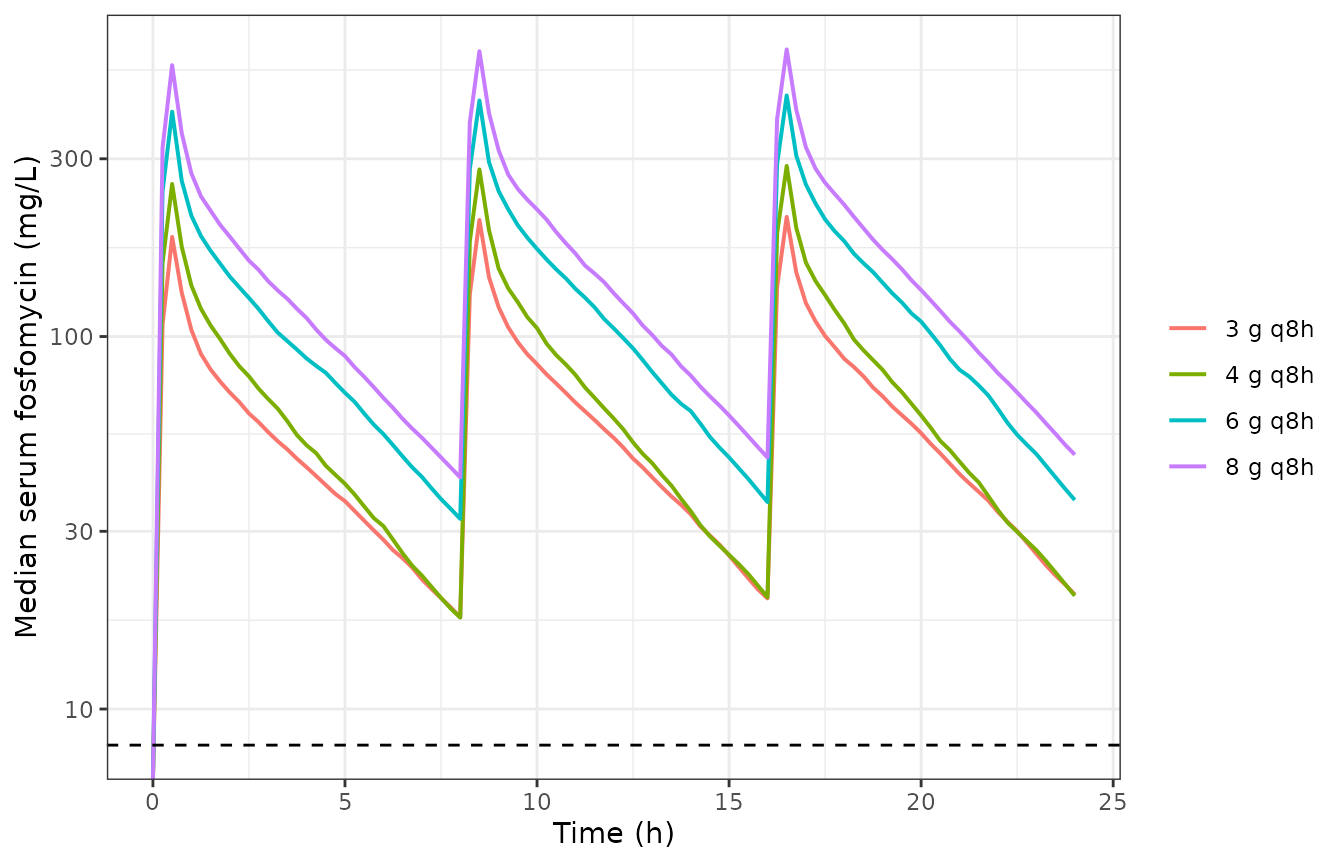
Replicates Figure 4 of Ortiz Zacarias 2018: median simulated serum fosfomycin after 3, 4, 6 and 8 g intravenously every 8 h (30-minute infusions). Dashed line is the E. coli epidemiological cut-off MIC of 8 mg/L.
Figure 5: oral regimens at 3 and 6 g
Figure 5 compares single-dose, twice-daily and three-times-daily oral regimens at 3 and 6 g. Its message is that only the tid arms hold above the MIC across the whole day.
oralGrid <- tidyr::expand_grid(dose_g = c(3, 6), ii = c(24, 12, 8))
oralArms <- lapply(seq_len(nrow(oralGrid)), function(k) {
  makeArm(
    oralGrid$dose_g[k] * 1000, oralGrid$ii[k], "depot",
    sprintf("%g g q%gh", oralGrid$dose_g[k], oralGrid$ii[k]),
    idOffset = (k - 1L) * N_PER_ARM
  )
})
#> Warning: 'ii' requires non zero additional doses ('addl') or steady state
#> dosing ('ii': 24.000000, 'ss': 0; 'addl': 0), reset 'ii' to zero
#> Warning: 'ii' requires non zero additional doses ('addl') or steady state
#> dosing ('ii': 24.000000, 'ss': 0; 'addl': 0), reset 'ii' to zero
oralSimCohort <- solveArms(po, oralArms)

oralSimCohort |>
  dplyr::group_by(treatment, time) |>
  dplyr::summarise(med = stats::median(Cc), .groups = "drop") |>
  dplyr::mutate(dose = sub(" .*", " g", treatment)) |>
  ggplot2::ggplot(ggplot2::aes(time, med, colour = treatment)) +
  ggplot2::geom_line(linewidth = 0.7) +
  ggplot2::geom_hline(yintercept = 8, linetype = "dashed") +
  ggplot2::facet_wrap(~dose) +
  ggplot2::labs(x = "Time (h)", y = "Median serum fosfomycin (mg/L)", colour = NULL) +
  ggplot2::theme_bw()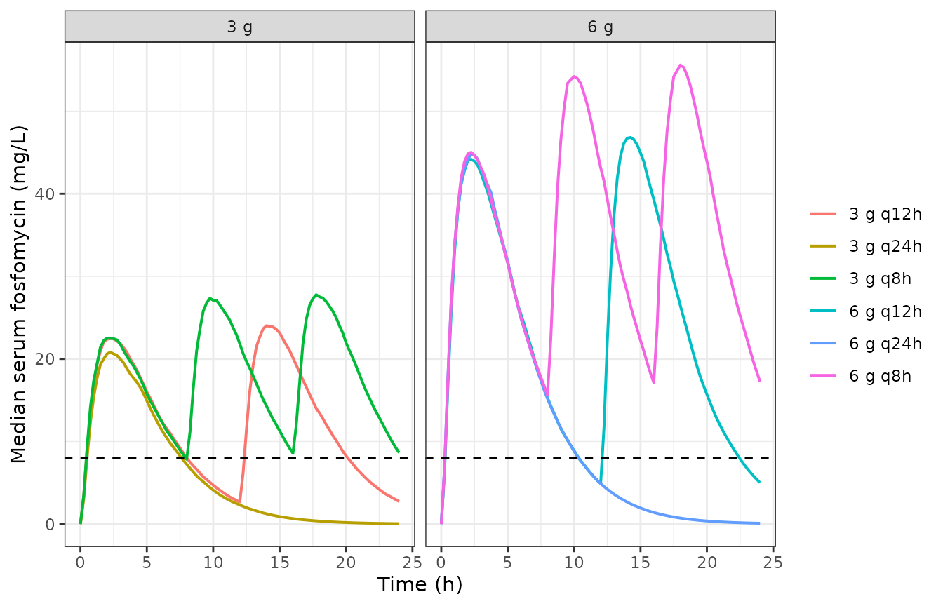
Replicates Figure 5 of Ortiz Zacarias 2018: median simulated serum fosfomycin after oral fosfomycin tromethamine 3 or 6 g given once (q24h), twice (q12h) or three times (q8h) daily. Dashed line is the MIC of 8 mg/L.
Figure 3: single oral doses with the full uncertainty layer
Figure 3 of the source shows the 90% prediction interval around
single 2 g and 5 g oral doses. Reproducing its width needs the
parameter-uncertainty layer of Equations 2 to 4 as well as IIV, which is
added here through thetaMat.
singleEv <- do.call(rbind, lapply(c(2, 5), function(d) {
  ev <- rxode2::et(amt = d * 1000, cmt = "depot")
  ev <- rxode2::et(ev, seq(0, 24, by = 0.5))
  ev <- as.data.frame(ev)
  ev$CRCL <- 103
  ev$treatment <- sprintf("%g g single oral dose", d)
  ev
}))

uncSim <-
  rxode2::rxSolve(
    po,
    events = singleEv,
    thetaMat = thetaMat,
    nStud = 40L,
    nSub = 5L,
    dfSub = 0, dfObs = 0,
    keep = "treatment",
    returnType = "data.frame"
  )

uncSim |>
  dplyr::group_by(treatment, time) |>
  dplyr::summarise(
    lo = stats::quantile(Cc, 0.05),
    med = stats::median(Cc),
    hi = stats::quantile(Cc, 0.95),
    .groups = "drop"
  ) |>
  ggplot2::ggplot(ggplot2::aes(time, med)) +
  ggplot2::geom_ribbon(ggplot2::aes(ymin = lo, ymax = hi), alpha = 0.25) +
  ggplot2::geom_line(linewidth = 0.7) +
  ggplot2::geom_hline(yintercept = 8, linetype = "dashed") +
  ggplot2::facet_wrap(~treatment) +
  ggplot2::labs(x = "Time (h)", y = "Serum fosfomycin (mg/L)") +
  ggplot2::theme_bw()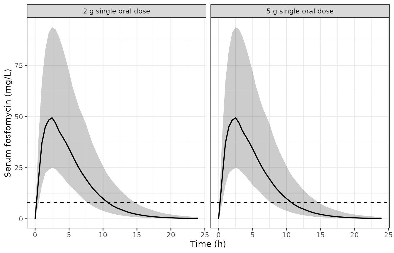
Replicates Figure 3B-C of Ortiz Zacarias 2018: median (line) and 90% prediction interval (band) of simulated serum fosfomycin after single oral doses of 2 g and 5 g, with parameter uncertainty (Equations 2-4, via thetaMat) and IIV both active. Dashed line is the MIC of 8 mg/L.
The band is wide, which is the source paper’s own conclusion about its model: “As all data points lie within the 90% PI of the simulations, the PI is wider than expected based on the data, indicating that the variability of the model is overestimated” (Section 3.1).
Assumptions and deviations
kb is an oral-model parameter only.
This is the load-bearing structural reading of the paper and the
arithmetic that settles it is worth recording. Table 2’s intravenous AUC
over 24 h at 3 g q8h is 1490.82 mg/Lh for a daily dose of 9000 mg,
implying a total elimination clearance of about 6.04 L/h – consistent
with CL = 5.808 L/h alone. Adding
kb * Vc = 5.05 L/h would give 10.86 L/h and an AUC near
829, which is 44% below the published value. Running the oral model
without* kb overshoots Table 3 in the other direction
(Cmax 46.5 against 28.44, AUC 894 against 475.42). Only the split
reading reproduces both tables, and it is what Section 2.1 says in
words.
Intravenous Cmax is not reproduced, and is excluded from the
gate. At the 30-minute infusion stated in Section 3.2, the
model gives a steady-state Cmax 41.9% above Table 2 for every q8h
regimen and 36.1% above for every q6h regimen. The offset is constant
across doses, so it is not a transcription error in a dose or a volume,
and AUC – which depends on dose and CL only, not on the infusion
duration – matches to 3.9%. The cause is that the paper prints
no numeric value for either Qinf or
tinf: Figure 1 parameterises the intravenous input
by those two symbols and Table 1 lists neither. Two readings were
tested. A zero-order 30-minute infusion (the natural reading of the
prose) gives +41.9%. A first-order input with rate constant
Qinf = 1 / tinf = 2 /h (the natural reading of the Figure 1
legend, which calls Qinf an “infusion rate
constant”) gives Cmax 137.5 against 151.41, or -9.2%, with AUC
within 0.9%. A zero-order infusion of about 1.55 h would reproduce Table
2’s Cmax exactly. Neither documented reading reproduces it, so the model
file encodes no infusion at all – the infusion is supplied by the user’s
event table, as it must be – and this vignette uses the 30-minute
reading the prose states while reporting the gap rather than tuning to
close it. Users reproducing Table 2’s Cmax specifically should be aware
of the ambiguity.
AUC window. Section 2.5 defines the tabulated AUC as “over a period of 24 hours at steady state”, which is what is computed above. For the q8h intravenous rows an AUC over the first 24 h instead matches more closely (-0.6% rather than +3.9%); the paper does not say which of the two its Table 2 used, and both are within 4%.
Table 3 q12h and q24h rows. These reproduce to 4.1-7.4% against 0.1-0.6% for the q8h rows. Fosfomycin’s terminal half-life here is about 2.6 h, so accumulation at a 12 or 24 h interval is negligible and the difference is not a steady-state artefact of this vignette; it most likely reflects the paper’s Monte Carlo summary statistic rather than a structural disagreement. The difference is well inside the gate and is recorded rather than tuned away.
No residual error. The paper reports no
residual-error model anywhere; its prediction intervals come from
parameter uncertainty and IIV alone. Both model files encode
addSd <- fixed(0) rather than inventing a magnitude. A
user refitting either model to real data must supply a residual-error
estimate.
Parameter uncertainty is not in ini().
Equations 2 to 4 are a simulation protocol above the model, so the
packaged models carry typical values and IIV only. The
thetaMat recipe above restores the layer. One nuance:
Equation 2 makes exp(theta_p,LN) the median of the
uncertainty distribution and theta_p,N its mean,
whereas ini() sets the median to the published
theta_p,N. The two differ by
exp(omega2_LN / 2), which is 2.2% for CL and
under 4% for the other three.
Equation 4 as printed does not draw a random number.
It reads theta_TV = exp(theta_p,LN + omega2_LN), which is
deterministic and, given Equation 2, equals
theta_p,N * exp(omega2_LN / 2). Section 2.3 nevertheless
says the typical values were “randomly sampled using the distributions
for parameter uncertainty”, so the printed Equation 4 is read here as a
typo for a draw from Normal(theta_p,LN, omega2_LN) in the
log domain. This was confirmed against a 300 dpi rendering of the page
rather than a text extraction, because pdftotext is known
to drop operators from display equations.
CLCR truncation bounds. Section 2.2 says the
simulated creatinine clearance was “limited between the minimal and
maximal reported values” of Sauermann et al., but neither bound is
printed in this paper. The virtual cohort above truncates at mean +/- 2
SD (21 to 185 mL/min) as a stand-in. This affects only the illustrative
figures; every quantitative gate is evaluated at the reference
CRCL = 103.
Population metadata. n_subjects records
the size of the upstream cohorts whose data the parameters actually rest
on (12 for the intravenous model, 12 + 5 for the oral model), not the
1000 virtual subjects Ortiz Zacarias 2018 simulated and not a cohort
this paper studied.
Salt forms. Doses are simulated in mg of fosfomycin as the paper states them, with no salt correction: Table 2 is labelled fosfomycin disodium and Table 3 fosfomycin tromethamine, and the paper applies no conversion factor to either.
No errata. A search of the publisher’s correction feed and PubMed found no erratum or corrigendum for this article.