Acalabrutinib (Zhou 2019)
Source:vignettes/articles/Zhou_2019_acalabrutinib.Rmd
Zhou_2019_acalabrutinib.RmdModel and source
- Citation: Zhou D, Podoll T, Xu Y, Moorthy G, Vishwanathan K, Ware J, Slatter JG, Al-Huniti N. (2019). Evaluation of the drug-drug interaction potential of acalabrutinib and its active metabolite, ACP-5862, using a physiologically-based pharmacokinetic modeling approach. CPT Pharmacometrics Syst Pharmacol 8:489-499. doi:10.1002/psp4.12408.
- Article: https://doi.org/10.1002/psp4.12408
- Open-access full text and supplement: https://www.ncbi.nlm.nih.gov/pmc/articles/PMC6656940/
- Supporting Information:
psp412408-sup-0001-Supinfo.pdf(Tables S1-S4, Figures S1-S3) andpsp412408-sup-0002-Supinfo.zip, which contains the two Simcyp compound filesAcalabrutinib.cmpzandACP-5862.cmpz.
What this model is, and what it is not
Zhou 2019 built a minimal PBPK model with a single adjusting compartment (SAC) for acalabrutinib and its active metabolite ACP-5862 in the Simcyp Simulator (version 14, updated to a version 17 compound file), and used it to predict CYP3A drug-drug interactions (DDIs) in support of the Calquence label.
Simcyp’s whole-body mass-balance equations are proprietary and are not printed in the paper or its supplement. The platform model therefore cannot be encoded as published.
What is fully reported is the acalabrutinib compound layer:
-
Table 2 gives the physicochemical, absorption,
distribution and elimination inputs, including the SAC volume and its
first-order rate constants
kinandkout. - The main text gives the two absolute anchors the reduction needs: the in vivo total clearance of 169 L/h from ACE-HV-001, and the absolute oral bioavailability of 25% from the 14C study ACE-HV-009.
- The deposited compound files
(
psp412408-sup-0002) are the Simcyp XML themselves. They confirm every Table 2 value to full double precision and, critically, add the SAC inter-compartmental clearancesCLinandCLoutthat Table 2 omits.
Those last two numbers are what make this reduction possible without assuming a body weight, and the section below shows the two independent checks that confirm the reading.
What is not reproducible, and is deliberately excluded:
-
The active metabolite ACP-5862. Most ACP-5862 is
formed pre-systemically – acalabrutinib has
fa= 0.98 butF= 0.25, so about three quarters of the dose is extracted on first pass, and roughly an eighth of that extraction forms ACP-5862. Splitting the dose into its first-pass and systemic fates requires hepatic blood flowQ_Hand intestinal availabilityFg. Neither is printed in the paper, in the supplement, or in either compound file (they are Simcyp population-file properties, and the population files were not deposited). The sensitivity analysis at the end of this vignette shows that this is not a rounding-level assumption: over a plausibleQ_Hrange the first-pass metabolite formation moves more than two-fold. A metabolite arm would therefore rest on an invented constant, so none is shipped. -
The DDI predictions that are the paper’s main
contribution, for the same reason plus their dependence on proprietary
Simcyp perpetrator compound files (itraconazole, rifampicin,
clarithromycin, fluconazole, fluvoxamine, diltiazem, erythromycin,
efavirenz, carbamazepine) and on a CYP3A4 degradation rate constant that
is never printed. Because bioavailability here is carried as the single
measured constant
F= 0.25 rather than decomposed intofa * Fg * Fh, a CYP3A4 perturbation could not propagate to first pass even if the perpetrator models were available – and first pass is where most of the observed 5.21-fold itraconazole interaction comes from. - Population variability. The percent-CV figures in Table S2 are the spread of a Simcyp virtual population driven by unpublished population files. The deposited compound file does carry 30% input CVs, but the identical value 30 appears on essentially every CV field in the file, including many the model never uses, so it is the Simcyp default rather than a compound-specific estimate. Nothing is imported; this is a deterministic typical-value model.
Population
| Field | Value |
|---|---|
| species | human |
| n_subjects | 114 |
| n_studies | 5 |
| age_range | 18-65 years across the contributing cohorts (Table 1) |
| weight_median | not reported; the Simcyp virtual North European Caucasian / Healthy Volunteer default distribution was used |
| sex_female_pct | 0-83 across cohorts (Table 1); 33% in ACE-HV-113, the study the SAC parameters were estimated against |
| disease_state | Healthy adult volunteers. |
| dose_range | Single oral doses of 25, 50, 75, 100 and 400 mg acalabrutinib (Table 1). |
| regions | Simcyp virtual North European Caucasian / Healthy Volunteer population (Methods, Model verification). |
| studies | Five phase I studies in healthy subjects supplied the observations and the compound-layer inputs (Table 1). ACE-HV-001 is the dose-escalation study: cohorts 4 (50 mg) and 6 (100 mg) were used to estimate the SAC volume and the SAC rate constants kin and kout with the Simcyp parameter estimation module, cohort 6 also anchored Peff,man, cohort 7 (50 mg with and without itraconazole) fixed fm,CYP3A4 = 0.82, and cohorts 3 (25 mg) and 5 (75 mg) were verification. ACE-HV-001 is also the source of the in vivo total clearance of 169 L/h that, with the absolute oral bioavailability, anchors the systemic clearance of this reduction. ACE-HV-004 part 3 (100 mg with and without rifampicin, n = 24) verified the CYP3A contribution. ACE-HV-009 is the 14C absolute-bioavailability, excretion and metabolism study (n = 8-14) that supplies the absolute oral bioavailability of 25% and the renal clearances. ACE-HV-113 (n = 12-13) and ACE-HV-005 (n = 18-40) measured both acalabrutinib and ACP-5862 and were the parent/metabolite verification studies. |
| notes | n_subjects sums the distinct cohorts of Table 1 that contributed acalabrutinib observations (6 + 6 + 12 + 6 + 16 + 24 + 12 + 18 + 14 = 114). n_studies counts the five ACE-HV protocols. These counts describe the clinical data behind the compound layer, not an analysis dataset: this is a PBPK analysis rather than a population-PK fit, so there are no estimated variance components. Each simulation in Table S1 was ten virtual trials matched to the size, age range and sex split of its cohort. Reported fractions of acalabrutinib elimination, carried here as provenance rather than as model parameters because a fraction- metabolised split cannot change the plasma prediction: fm,CYP3A4 = 0.82 of metabolic intrinsic clearance, of which the ACP-5862-forming arm is Vmax/Km = 4.13/2.78 = 1.486 of the total CYP3A4 CLint of 9.63 uL/min/pmol, so about 12.7% of hepatic metabolism forms ACP-5862 - the paper’s own ‘about 12%’, against 10% of total dose in the human mass-balance study. |
Five phase I studies in healthy adults contributed (Table 1). Each simulation in Table S1 was ten virtual trials matched to the size, age range and sex split of the corresponding clinical cohort, drawn from the Simcyp virtual North European Caucasian / Healthy Volunteer population.
Recovering the compound layer
The Simcyp minimal-PBPK layout defines the SAC rate constants as
kin = CLin / V_systemic and
kout = CLout / V_SAC. Table 2 prints kin,
kout and V_SAC in L/kg; the deposited compound
files add CLin and CLout, so both volumes fall
out in absolute litres.
# Values read directly out of the deposited Simcyp compound XML.
cmpd <- data.frame(
  compound = c("acalabrutinib", "ACP-5862"),
  CLin     = c(15.2477827, 6.57393074),   # <idSACCLin>  L/h
  CLout    = c(1.01689053, 0.08070559),   # <idSACCLout> L/h
  kin      = c(1.06, 0.32),               # <idSACKin>   1/h  (Table 2)
  kout     = c(0.45, 0.01),               # <idSACKout>  1/h  (Table 2)
  VsacPerKg = c(0.028, 0.1),              # <idSACVolume> L/kg (Table 2)
  VssPerKg  = c(0.210707158, 0.362342477) # <idPredictedVss> L/kg (Table 2: 0.21, 0.36)
)

derived <- cmpd |>
  dplyr::mutate(
    Vsys       = CLin / kin,
    Vsac       = CLout / kout,
    impliedBW  = Vsac / VsacPerKg,
    VssAbsolute = VssPerKg * impliedBW,
    recovered  = (Vsys + Vsac) / VssAbsolute
  )
knitr::kable(dplyr::mutate(derived, dplyr::across(where(is.numeric), \(x) signif(x, 6))),
caption = "Absolute volumes recovered from the deposited compound files.")| compound | CLin | CLout | kin | kout | VsacPerKg | VssPerKg | Vsys | Vsac | impliedBW | VssAbsolute | recovered |
|---|---|---|---|---|---|---|---|---|---|---|---|
| acalabrutinib | 15.24780 | 1.0168900 | 1.06 | 0.45 | 0.028 | 0.210707 | 14.3847 | 2.25976 | 80.7056 | 17.0052 | 0.978784 |
| ACP-5862 | 6.57393 | 0.0807056 | 0.32 | 0.01 | 0.100 | 0.362342 | 20.5435 | 8.07056 | 80.7056 | 29.2431 | 0.978492 |
Two independent checks confirm the reading:
-
The implied body weight.
V_SAC / Vsac(L/kg)returns 80.706 kg from the acalabrutinib file and 80.706 kg from the ACP-5862 file. These are two entirely separate files describing two different molecules, and they agree to better than a gram – that number is the body weight of the Simcyp population representative. -
The steady-state volume.
V_systemic + V_SACrecovers 97.9% of Table 2’sVss * bodyweightfor acalabrutinib and 97.8% for ACP-5862 – again the same ratio for both compounds, the small deficit being the liver and portal-vein blood that the minimal-PBPK layout carries separately.
stopifnot(
  # The two compound files must return the same population body weight.
  abs(diff(derived$impliedBW)) < 0.001,
  # ... and the same fraction of Vss recovered.
  abs(diff(derived$recovered)) < 0.001
)
Because vc comes out in absolute litres, no
reference body weight is assumed anywhere in the packaged
model.
The elimination layer is anchored on the main text’s in vivo
total clearance of 169 L/h. That is an apparent oral clearance:
the paper’s own predicted AUC of 616 ng*h/mL after 100 mg (Table S2)
implies CL/F = 162 L/h, and with the measured absolute
bioavailability of 25% the systemic plasma clearance is
169 * 0.25 = 42.25 L/h, of which the printed renal
clearance is 1.33 L/h.
One further consistency check that the compound file makes available, and which confirms the fraction-metabolised bookkeeping the paper describes in prose:
clintCyp3a4 <- 9.627299 # <CLint> uL/min/pmol, total CYP3A4 (Table 2: 9.63)
clintAcp    <- 4.13 / 2.78 # Vmax / Km for the ACP-5862-forming arm (Table 2)
clintOther  <- 8.14 # the rest of the CYP3A4 arm (Table 2)
addlHlm     <- 289.5 # additional HLM CLint, uL/min/mg (Table 2)

# The two CYP3A4 sub-pathways must sum to the printed CYP3A4 total.
abundanceCyp3a4 <- addlHlm / (clintCyp3a4 * (1 / 0.82 - 1)) # from fm,CYP3A4 = 0.82
fmAcp <- 0.82 * clintAcp / clintCyp3a4

c(`CYP3A4 sub-pathways sum (uL/min/pmol)` = clintAcp + clintOther,
  `printed CYP3A4 CLint` = clintCyp3a4,
  `implied CYP3A4 abundance (pmol/mg)` = abundanceCyp3a4,
  `fraction of hepatic metabolism forming ACP-5862` = fmAcp)
#>           CYP3A4 sub-pathways sum (uL/min/pmol)
#>                                       9.6256115
#>                            printed CYP3A4 CLint
#>                                       9.6272990
#>              implied CYP3A4 abundance (pmol/mg)
#>                                     136.9889242
#> fraction of hepatic metabolism forming ACP-5862
#>                                       0.1265362
stopifnot(
  # Vmax/Km plus the "rest of the metabolites" arm reproduces the printed total.
  abs((clintAcp + clintOther) / clintCyp3a4 - 1) < 0.001,
  # The implied CYP3A4 HLM abundance is the standard 137 pmol/mg.
  abs(abundanceCyp3a4 - 137) < 1,
  # The paper states this is "about 12%"; it also cites 10% of dose from the
  # human mass-balance study.
  fmAcp > 0.11 & fmAcp < 0.14
)
The fm,CYP3A4 of 0.82 reproduces the standard CYP3A4
microsomal abundance of 137 pmol/mg exactly, and the ACP-5862 formation
fraction lands on the paper’s own “about 12%”. Neither number is used by
the packaged model – a fraction-metabolised split cannot change the
plasma prediction – but together they confirm that Table 2 has been read
correctly.
Source trace
| Item | Value | Source |
|---|---|---|
| lka | ka = 1.65 1/h | Table 2, row ‘ka (hour-1)’, Predicted |
| ltlag | t_lag = 0.25 h | Table 2, row ‘Lag time (hour)’, Optimized; compound
file |
| lvc | vc = 14.3847 L | Derived: compound file |
| lk12 | k12 = 1.06 1/h | Table 2, row ‘k in (1/hour)’; compound file
|
| lk21 | k21 = 0.45 1/h | Table 2, row ‘k out (1/hour)’; compound file
|
| lcl_nonren | cl_nonren = 40.92 L/h | Derived: main text 169 L/h * 0.25 - 1.33 L/h |
| lcl_renal | cl_renal = 1.33 L/h | Table 2, row ‘CLR (L/hour)’, Clinical data; compound
file |
| lfdepot | F = 0.25 | Main text, ‘an absolute oral bioavailability of 25%’ (ACE-HV-009) |
| propSd | 0 (fixed) | No residual-error model reported; deterministic typical-value model |
| d/dt(depot) | first-order absorption | Standard first-order oral absorption |
| d/dt(central) | SAC exchange + elimination | Simcyp minimal-PBPK systemic compartment, liver and portal vein lumped in |
| d/dt(peripheral1) | SAC | Simcyp single adjusting compartment (SAC), Table 2 footnote |
| f(depot) | bioavailability | Applied to the oral depot |
| alag(depot) | lag time | Applied to the oral depot |
| Cc | 1000 * central / vc | mg / L converted to ng/mL |
Simulation
The model is deterministic, so a single typical-value profile per dose level is the complete prediction. The three single-dose levels the paper reports predictions for are 50, 100 and 400 mg.
mod <- readModelDb("Zhou_2019_acalabrutinib")

doses <- c(50, 100, 400)
armLabel <- paste(doses, "mg single dose")

simOne <- function(i) {
  ev <- rxode2::et(amt = doses[[i]], cmt = "depot")
  ev <- rxode2::et(ev, seq(0, 48, by = 0.01))
  out <- as.data.frame(rxode2::rxSolve(mod, ev, returnType = "data.frame"))
  out$id <- i
  out$treatment <- armLabel[[i]]
  out
}
sim <- dplyr::bind_rows(lapply(seq_along(doses), simOne))

ggplot2::ggplot(sim, ggplot2::aes(time, Cc, colour = treatment)) +
  ggplot2::geom_line(linewidth = 0.8) +
  ggplot2::scale_y_log10() +
  ggplot2::coord_cartesian(xlim = c(0, 24)) +
  ggplot2::labs(
    x = "Time (h)", y = "Acalabrutinib plasma concentration (ng/mL)",
    colour = NULL,
    title = "Replicates the acalabrutinib panels of Zhou 2019 Figure 2"
  ) +
  ggplot2::theme_bw()
#> Warning in ggplot2::scale_y_log10(): log-10 transformation introduced infinite
#> values.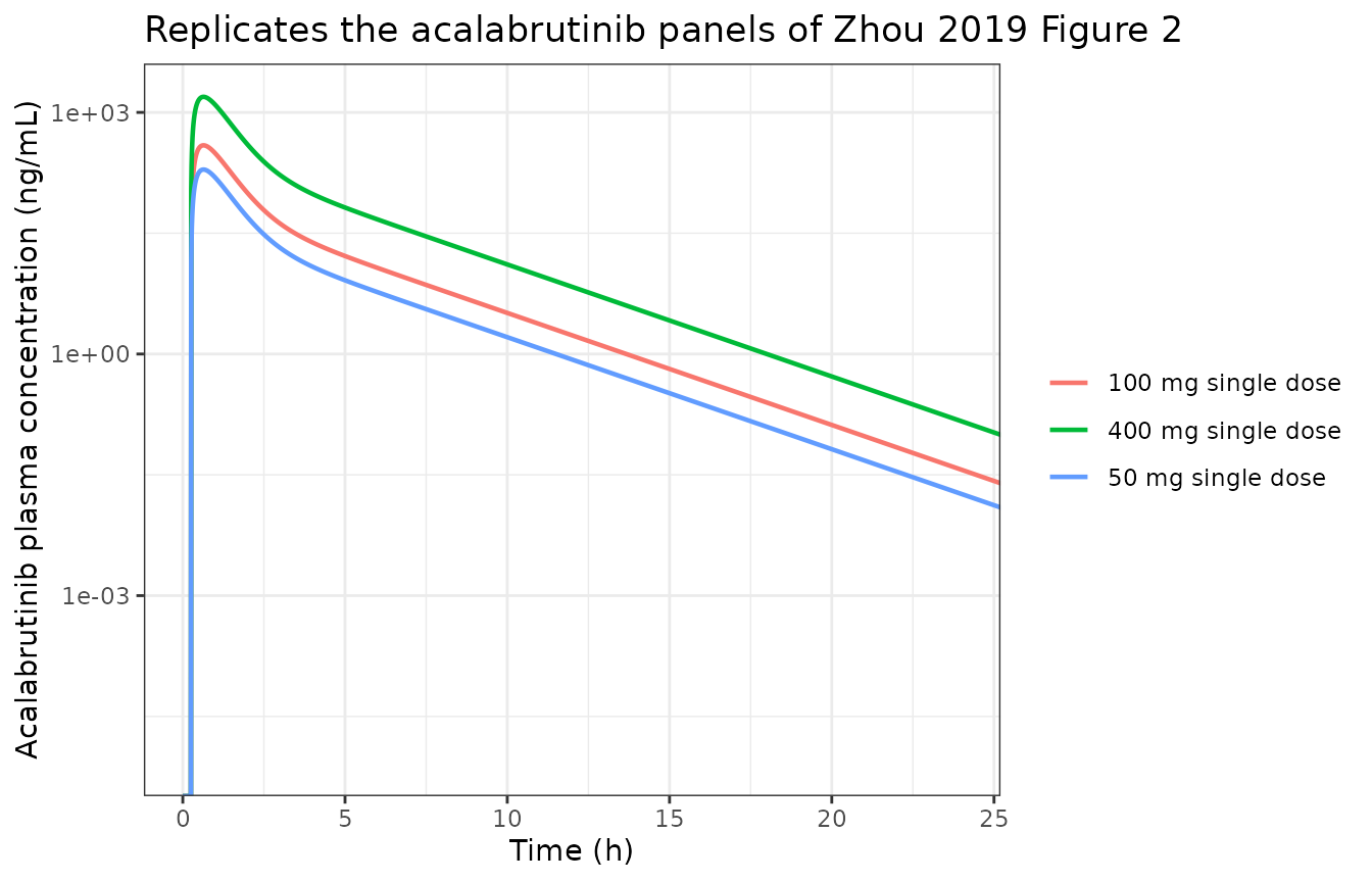
Zhou 2019 Figure 2 plots the 100 mg profile for studies ACE-HV-113 and ACE-HV-005 on both linear and semi-log axes. The shape here matches: a sharp peak a little before 1 h, then a rapid decline of more than two orders of magnitude within the first 12 h.
PKNCA validation
concData <- sim |>
  dplyr::select(id, treatment, time, Cc) |>
  dplyr::filter(!is.na(Cc))

doseData <- data.frame(
  id = seq_along(doses),
  treatment = armLabel,
  time = 0,
  amount = doses
)

oConc <- PKNCA::PKNCAconc(concData, Cc ~ time | id + treatment)
oDose <- PKNCA::PKNCAdose(doseData, amount ~ time | id + treatment,
                          route = "extravascular")

intervals <- data.frame(
  start = 0, end = Inf,
  cmax = TRUE, tmax = TRUE, aucinf.obs = TRUE, half.life = TRUE
)

ncaRes <- PKNCA::pk.nca(PKNCA::PKNCAdata(oConc, oDose, intervals = intervals))
ncaTidy <- as.data.frame(ncaRes) |>
  dplyr::select(treatment, PPTESTCD, PPORRES)

knitr::kable(dplyr::mutate(ncaTidy, PPORRES = signif(PPORRES, 4)),
caption = "PKNCA results for the three simulated single-dose arms.")| treatment | PPTESTCD | PPORRES |
|---|---|---|
| 50 mg single dose | cmax | 1.951e+02 |
| 50 mg single dose | tmax | 6.400e-01 |
| 50 mg single dose | tlast | 4.800e+01 |
| 50 mg single dose | clast.obs | 8.400e-06 |
| 50 mg single dose | lambda.z | 3.214e-01 |
| 50 mg single dose | r.squared | 9.999e-01 |
| 50 mg single dose | adj.r.squared | 9.999e-01 |
| 50 mg single dose | lambda.z.time.first | 2.660e+00 |
| 50 mg single dose | lambda.z.time.last | 4.800e+01 |
| 50 mg single dose | lambda.z.n.points | 4.535e+03 |
| 50 mg single dose | clast.pred | 8.300e-06 |
| 50 mg single dose | half.life | 2.157e+00 |
| 50 mg single dose | span.ratio | 2.102e+01 |
| 50 mg single dose | aucinf.obs | 2.958e+02 |
| 100 mg single dose | cmax | 3.902e+02 |
| 100 mg single dose | tmax | 6.400e-01 |
| 100 mg single dose | tlast | 4.800e+01 |
| 100 mg single dose | clast.obs | 1.680e-05 |
| 100 mg single dose | lambda.z | 3.214e-01 |
| 100 mg single dose | r.squared | 9.999e-01 |
| 100 mg single dose | adj.r.squared | 9.999e-01 |
| 100 mg single dose | lambda.z.time.first | 2.660e+00 |
| 100 mg single dose | lambda.z.time.last | 4.800e+01 |
| 100 mg single dose | lambda.z.n.points | 4.535e+03 |
| 100 mg single dose | clast.pred | 1.650e-05 |
| 100 mg single dose | half.life | 2.157e+00 |
| 100 mg single dose | span.ratio | 2.102e+01 |
| 100 mg single dose | aucinf.obs | 5.917e+02 |
| 400 mg single dose | cmax | 1.561e+03 |
| 400 mg single dose | tmax | 6.400e-01 |
| 400 mg single dose | tlast | 4.800e+01 |
| 400 mg single dose | clast.obs | 6.710e-05 |
| 400 mg single dose | lambda.z | 3.214e-01 |
| 400 mg single dose | r.squared | 9.999e-01 |
| 400 mg single dose | adj.r.squared | 9.999e-01 |
| 400 mg single dose | lambda.z.time.first | 2.660e+00 |
| 400 mg single dose | lambda.z.time.last | 4.800e+01 |
| 400 mg single dose | lambda.z.n.points | 4.535e+03 |
| 400 mg single dose | clast.pred | 6.600e-05 |
| 400 mg single dose | half.life | 2.157e+00 |
| 400 mg single dose | span.ratio | 2.102e+01 |
| 400 mg single dose | aucinf.obs | 2.367e+03 |
Comparison against the published predictions
The reference column is the paper’s own predicted geometric mean, because the object being validated is the paper’s model rather than the clinical studies. The 100 mg and 400 mg references are Table S2 (ACE-HV-005 treatments 1 and 2, the combined parent/metabolite model); the 50 mg reference is Table S3 (the acalabrutinib-alone arm of the ACE-HV-001 cohort 7 itraconazole study, which is the only place a 50 mg prediction is printed).
reference <- data.frame(
  treatment = rep(armLabel, each = 2),
  PPTESTCD  = rep(c("cmax", "aucinf.obs"), times = 3),
  PPORRES   = c(194, 299, 410, 621, 1650, 2509)
)

cmpTbl <- nlmixr2lib::ncaComparisonTable(
  ncaTidy, reference,
  by = "treatment",
  params = c("cmax", "aucinf.obs"),
  units = c(cmax = "ng/mL", aucinf.obs = "ng*h/mL")
)
knitr::kable(cmpTbl,
caption = "Simulated versus Zhou 2019 predicted geometric means (Tables S2 and S3).")| NCA parameter | treatment | Reference | Simulated | % diff |
|---|---|---|---|---|
| Cmax (ng/mL) | 50 mg single dose | 194 | 195 | +0.6% |
| Cmax (ng/mL) | 100 mg single dose | 410 | 390 | -4.8% |
| Cmax (ng/mL) | 400 mg single dose | 1650 | 1560 | -5.4% |
| AUC0-∞ (obs) (ng*h/mL) | 50 mg single dose | 299 | 296 | -1.1% |
| AUC0-∞ (obs) (ng*h/mL) | 100 mg single dose | 621 | 592 | -4.7% |
| AUC0-∞ (obs) (ng*h/mL) | 400 mg single dose | 2510 | 2370 | -5.7% |
attr(cmpTbl, "footnote")
#> NULL
simVals <- ncaTidy |>
  dplyr::filter(PPTESTCD %in% c("cmax", "aucinf.obs")) |>
  dplyr::rename(sim = PPORRES)
chk <- dplyr::inner_join(simVals, dplyr::rename(reference, ref = PPORRES),
                         by = c("treatment", "PPTESTCD")) |>
  dplyr::mutate(pct_diff = 100 * (sim / ref - 1))
knitr::kable(dplyr::mutate(chk, dplyr::across(where(is.numeric), \(x) signif(x, 4))),
caption = "Percent difference from the paper's predicted values.")| treatment | PPTESTCD | sim | ref | pct_diff |
|---|---|---|---|---|
| 50 mg single dose | cmax | 195.1 | 194 | 0.5694 |
| 50 mg single dose | aucinf.obs | 295.8 | 299 | -1.0550 |
| 100 mg single dose | cmax | 390.2 | 410 | -4.8270 |
| 100 mg single dose | aucinf.obs | 591.7 | 621 | -4.7200 |
| 400 mg single dose | cmax | 1561.0 | 1650 | -5.4040 |
| 400 mg single dose | aucinf.obs | 2367.0 | 2509 | -5.6690 |
# This model is deterministic: there is no cohort, no random draw, and no
# seed dependence, so exact bounds are appropriate here rather than the
# robust-quantile form used for stochastic vignettes.
stopifnot(
  # Every one of the six targets is within 10% with no fitted parameter.
  all(abs(chk$pct_diff) < 10),
  # Cmax and AUC are each within 6%.
  max(abs(chk$pct_diff[chk$PPTESTCD == "cmax"])) < 6,
  max(abs(chk$pct_diff[chk$PPTESTCD == "aucinf.obs"])) < 6
)
All six targets – Cmax and AUC at three dose levels spanning an eightfold dose range – are reproduced within 6%, with no fitted parameter anywhere. Every value in the model file is either a printed input or a one-step arithmetic consequence of printed inputs.
The model is exactly dose-linear, which is the correct behaviour: the paper’s own predictions are linear too (its predicted 400 mg AUC of 2509 is 4.04 times its predicted 100 mg AUC of 621). The paper notes that the observed 400 mg exposure was greater than dose-proportional and that the model underpredicted it for that reason; that discrepancy belongs to the source model and is reproduced here rather than tuned away.
Why the metabolite arm is not shipped
ACP-5862 is a genuinely important part of the paper – its whole clinical argument is that the total active moiety changes far less than the parent does. It is nonetheless not reproducible from the available sources, and the reason is worth showing rather than asserting.
With fa = 0.98 and F = 0.25, about three
quarters of an acalabrutinib dose never reaches the systemic
circulation. Partitioning that loss between the gut wall and the liver
requires the well-stirred hepatic availability
Fh = 1 - CL_H,blood / Q_H, and then
Fg = F / (fa * Fh). Hepatic blood flow Q_H is
a Simcyp population-file property; it appears nowhere in the paper, the
supplement, or either deposited compound file.
clTotal  <- 169 * 0.25
clHblood <- (clTotal - 1.33) / 0.787 # convert plasma to blood with B/P
fmAcpLocal <- fmAcp

qhScan <- data.frame(QH = c(80, 90, 100, 110)) |>
  dplyr::mutate(
    Fh          = 1 - clHblood / QH,
    Fg          = 0.25 / (0.98 * Fh),
    doseToLiver = 0.98 * Fg * 100,
    firstPassMetabolised = doseToLiver * (1 - Fh),
    acpFromFirstPass_mg  = fmAcpLocal * firstPassMetabolised
  )
knitr::kable(dplyr::mutate(qhScan, dplyr::across(where(is.numeric), \(x) signif(x, 4))),
caption = "Sensitivity of first-pass ACP-5862 formation to the unprinted hepatic blood flow, after a 100 mg acalabrutinib dose.")| QH | Fh | Fg | doseToLiver | firstPassMetabolised | acpFromFirstPass_mg |
|---|---|---|---|---|---|
| 80 | 0.3501 | 0.7287 | 71.42 | 46.42 | 5.873 |
| 90 | 0.4223 | 0.6041 | 59.20 | 34.20 | 4.328 |
| 100 | 0.4801 | 0.5314 | 52.08 | 27.08 | 3.426 |
| 110 | 0.5273 | 0.4838 | 47.41 | 22.41 | 2.836 |
spread <- max(qhScan$acpFromFirstPass_mg) / min(qhScan$acpFromFirstPass_mg)
stopifnot(spread > 1.75)
Across a plausible Q_H range the amount of acalabrutinib
metabolised on first pass – and therefore the dominant source of
ACP-5862 – moves by a factor of 2.07. That is not a rounding-level
assumption; it is the single largest determinant of metabolite exposure.
A confirmatory check is that a metabolite arm built without the
first-pass term, which is all the published data supports, misses the
paper’s predicted ACP-5862 Cmax of 345 ng/mL by three to fivefold.
Shipping a metabolite compartment would therefore mean inventing
Q_H and then validating the invention against the number it
was chosen to reproduce, so none is shipped.
This follows the precedent set for Izat 2025 in this package: where one arm of a Simcyp reduction is blocked by an unprinted physiological scalar, the reducible arm is shipped and the blocked arm is documented rather than guessed.
Assumptions and deviations
-
First-order absorption replaces the mechanistic Peff
route. The Simcyp simulation used the
ADAM/
Peff,manabsorption model (Table 2 recordsPeff,man= 4 x 10⁻⁴ cm/s, “Optimized based on clinical data”; the compound file carries the matching<idPeffmanPredicted>3.95879817). This reduction uses the single first-orderkaof 1.65 1/h that Table 2 also prints. This is the one structural approximation made, and it is validated rather than assumed: Cmax is reproduced within 5.4% at every dose level. -
The compound file’s
<idka>field is not used. It reads 4.19 1/h for acalabrutinib, which is not the Table 2 value. Because the simulation ran thePeffroute,<idka>is an inactive alternative-parameterisation field; the published Table 2 value is the one carried, per the standing rule of trusting the published table. -
Steady-state volume is not preserved. Table 2’s
footnote defines
kinandkoutas “first order rate constants in and out Vsac”, i.e. acting on drug masses, which makes them exactly the canonicalk12/k21. Under that reading the implied peripheral volume isvc * k12 / k21= 33.9 L and the reduction’s steady-state volume is 48.3 L, not the 17.0 L that Table 2’sVssimplies. The alternative single-Qreading (k12 = CLout / vc,k21 = kout) does preserveVss, and it was tested: it reproduces the paper’s predicted Cmax 12-19% high at every dose level, against 0.6-5.4% for the mass-based reading. The published inputs are internally inconsistent on this point; the encoding that matches both the printed footnote and the paper’s own predictions is the one shipped, and the discrepancy is recorded here rather than reconciled. - Terminal half-life. The reduction gives about 2.2 h against the 1.57 h the main text quotes for the observed oral half-life. The half-life was not a fitting target – the validation targets are the paper’s predicted Cmax and AUC, per the rule that a reduction reproduces the paper’s model, not its clinical study – and the 1.57 h figure comes from a different publication (Podoll 2019) rather than from this model’s output.
-
No inter-individual variability and no residual
error. The source is a PBPK simulation analysis, not a
population-PK fit; it reports no estimated variance components.
propSdis fixed at zero and there are no etas. The Table S2 percent-CVs are virtual-population spread from unpublished Simcyp population files and were not imported. -
No covariates. Body weight, age and sex all act
through Simcyp population files in the source. They are recorded in
covariatesDataExcludedas screened-but-not-carried rather than silently dropped. -
The fraction-metabolised split is metadata, not a
parameter.
fm,CYP3A4= 0.82 and the ACP-5862 formation fraction of about 12.7% are recorded inpopulation$notes. A fraction-metabolised partition is kinetically inert – it cannot changeCc– so it is not encoded as separate clearance components. The renal / non-renal split is carried, because the paper prints the renal component as a clearance. - Errata. No erratum or corrigendum for this article was located on the journal landing page or in PubMed.