Doxorubicin (Kunarajah 2017)
Source:vignettes/articles/Kunarajah_2017_doxorubicin.Rmd
Kunarajah_2017_doxorubicin.RmdModel and source
- Citation: Kunarajah K, Hennig S, Norris RLG, Lobb M, Charles BG, Pinkerton R, Moore AS. Population pharmacokinetic modelling of doxorubicin and doxorubicinol in children with cancer: is there a relationship with cardiac troponin profiles? Cancer Chemother Pharmacol. 2017;79(6):1209-1217. doi:10.1007/s00280-017-3309-6
- Article: https://doi.org/10.1007/s00280-017-3309-6
Population
Kunarajah 2017 enrolled 19 paediatric oncology patients aged 3.42-14.67 years (median 7.50) at the Royal Children’s Hospital, Brisbane, Australia; 17 contributed PK / cTnI samples (Table 1). Diagnoses were a mix of childhood malignancies (Hodgkin lymphoma, non-Hodgkin lymphoma, hepatoblastoma, Wilms’ tumour, T-ALL and Pre-B ALL, synovial sarcoma, neuroblastoma, osteosarcoma) treated with single IV doses of doxorubicin ranging 25-75 mg/m^2 (median 30 mg/m^2) given over infusion durations of 0.25-72.5 h. Body weight ranged 11.0-88.6 kg, height 0.9-1.8 m, and the sex split was 5 female / 12 male (29.4% female). 11 of the 17 patients had prior anthracycline exposure (median prior cumulative anthracycline-equivalent dose 100 mg/m^2, range 0-225 mg/m^2). Sampling covered 5-10 min, 1-2 h, 2-12 h, 24-120 h, and 168 h post-dose, yielding 99 doxorubicin, 119 doxorubicinol, and 104 cTnI concentrations for the population fit. Lower limit of quantification was 4.7 ng/mL for both analytes; the cTnI assay’s positive-leak threshold was 0.04 ug/L.
The same information is available programmatically via
rxode2::rxode(readModelDb("Kunarajah_2017_doxorubicin"))$population.
Source trace
Final parameter estimates and equations come from Kunarajah 2017 (Table 2 + Appendix NM-TRAN control stream). Fixed parameters carried from the upstream Kontny 2013 doxorubicin popPK fit (reference 12 in the paper) are flagged.
| Equation / parameter | Value | Source location |
|---|---|---|
lcl (CL) |
58.7 L/h/1.8 m^2 | Table 2 row 1; Appendix THETA(1) |
lvc (V1) |
32.2 L/1.8 m^2 | Table 2 row 2; Appendix THETA(2) |
lq (Q2) |
35.8 L/h/1.8 m^2 FIX | Table 2 row 3 FIX; Appendix THETA(5) FIX |
lvp (V2) |
3810 L/1.8 m^2 FIX | Table 2 row 4 FIX; Appendix THETA(6) FIX |
lq2 (Q3) |
65.1 L/h/1.8 m^2 FIX | Table 2 row 5 FIX; Appendix THETA(7) FIX |
lvp2 (V3) |
705 L/1.8 m^2 FIX | Table 2 row 6 FIX; Appendix THETA(8) FIX |
lqm (Qm formation CL) |
32.1 L/h/1.8 m^2 FIX | Table 2 row 9 FIX; Appendix THETA(13) FIX |
lcl_doxol (CLm) |
19.9 L/h/1.8 m^2 | Table 2 row 7; Appendix THETA(11) |
lvc_doxol (V4) |
508 L/1.8 m^2 | Table 2 row 8; Appendix THETA(12) |
e_age_cl (age-on-CL exponent) |
0.736 FIX | Table 2 row 10 FIX; Appendix THETA(9) FIX |
e_bsa_clvc (BSA linear coefficient) |
0.465 FIX | Table 2 row 11 FIX; Appendix THETA(10) FIX |
lkdeg (cTnI degradation) |
0.6 1/h | Table 2 row 12; Appendix THETA(16) |
lemax (cTnI Emax) |
0.15 | Table 2 row 14; Appendix THETA(19) |
lec50 (cTnI EC50) |
11.8 ug/L | Table 2 row 15; Appendix THETA(20) |
lbl_ctni (Cbase cTnI for PCAMT=90) |
0.021 ug/L (= 20.5 pg/mL) | Table 2 row 13; Appendix THETA(17); paper text p.6 |
e_pcamt_bl_ctni |
0.00308 per mg/m^2 (~0.31%) | Table 2 row 16; Appendix THETA(21); paper text p.6 |
| Proportional residual SD doxorubicin | 0.203 | Table 2; Appendix THETA(3) |
| Additive residual SD doxorubicin | 0.24 ug/L | Table 2; Appendix THETA(4) |
| Proportional residual SD doxorubicinol | 0.229 | Table 2; Appendix THETA(14) |
| Additive residual SD doxorubicinol | 0.95 ug/L | Table 2; Appendix THETA(15) |
| Proportional residual SD cTnI | 0.582 | Table 2; Appendix THETA(18) |
d/dt(central) 3-cmt IV with -CL/Vc |
– | Appendix $DES; Fig 2 schematic |
d/dt(central_doxol) Qm/Vc * central |
– | Appendix $DES; Fig 2 schematic |
Emax stimulation of ksyn
|
– | Eq. 1 page 4; Eqs. 2-3 page 4 |
BSA factor 1 + (BSA - 1.8) * 0.465
|
– | Table 2 footnote; Appendix FBSACL
|
Age factor 1 + (AGE/8.4)^0.736
|
– | Table 2 footnote; Appendix FAGE
|
PCAMT factor 1 + 0.00308*(PCAMT-90)
|
– | Table 2 footnote (Cbase_cTnI equation) |
The value column shows the typical-value parameter
estimate; the in-file comments next to each ini() entry pin
every value to the same locations.
Virtual cohort
set.seed(20170425) # Kunarajah 2017 published-online date

# Cohort patient characteristics from Table 1 (n = 17 with PK samples).
# We carry AGE, BSA (computed via Mosteller from height/weight), and
# PRIOR_ANTHRACYCLINE_DOSE per Kunarajah 2017 Table 1 directly.
cohort <- tibble::tribble(
  ~id, ~AGE, ~WT,  ~HT, ~PRIOR_ANTHRACYCLINE_DOSE, ~DOSE_MG_M2, ~INF_DUR_H,
   1L, 12.7, 40.0, 1.5,  225,                       25,         0.5,
   2L,  3.4, 12.8, 0.9,   90,                       30,         1.5,
   3L, 13.4, 60.0, 1.7,  120,                       60,         0.5,
   4L,  6.3, 20.5, 1.1,  100,                       50,         6.5,
   5L,  7.8, 28.3, 1.2,  200,                       33.3,       5.0,
   6L,  9.8, 31.3, 1.3,  100,                       25,         0.25,
   7L,  7.5, 25.5, 1.2,  125,                       25,         0.25,
   8L, 14.7, 62.7, 1.8,   75,                       75,         49.0,
   9L,  6.9, 20.6, 1.2,    0,                       25,         0.25,
  10L,  5.3, 16.9, 1.1,   25,                       25,         0.25,
  11L,  5.0, 11.0, 1.0,    0,                       75,         72.5,
  12L, 14.5, 37.3, 1.5,  120,                       30,         6.75,
  13L,  5.2, 25.0, 1.2,   50,                       25,         0.25,
  14L,  3.4, 17.0, 1.0,    0,                       75,         72.0,
  15L,  3.8, 17.0, 1.0,    0,                       60,         1.0,
  16L,  3.8, 14.0, 0.9,    0,                       75,         68.8,
  17L, 12.9, 88.6, 1.6,    0,                       75,         48.0
) |>
  mutate(
    BSA      = sqrt(WT * HT * 100 / 3600),                 # Mosteller BSA (m^2)
    DOSE_MG  = DOSE_MG_M2 * BSA,                           # absolute IV dose (mg)
    RATE_MGH = DOSE_MG / INF_DUR_H,                        # zero-order infusion rate (mg/h)
    PRIOR_GROUP = ifelse(PRIOR_ANTHRACYCLINE_DOSE > 0, ">0", "0")
  )

# Build the event table: one infusion per subject + a 168 h grid of obs
# times on Cc (rxSolve returns Cc, Cc_doxol, cTnI columns regardless of
# which named output the obs row's cmt is assigned to, so a single Cc
# observation row per time gives a one-row-per-time output frame).
obs_times <- c(seq(0.05, 6, length.out = 25),
               seq(8, 24, length.out = 9),
               seq(36, 168, length.out = 12))

events <- cohort |>
  rowwise() |>
  do({
    s <- .
    bind_rows(
      tibble(id = s$id, time = 0,                amt = s$DOSE_MG, dur = s$INF_DUR_H,
             evid = 1L, cmt = "central"),
      tibble(id = s$id, time = obs_times,        amt = NA_real_,  dur = NA_real_,
             evid = 0L, cmt = "Cc")
    ) |>
      mutate(BSA = s$BSA, AGE = s$AGE,
             PRIOR_ANTHRACYCLINE_DOSE = s$PRIOR_ANTHRACYCLINE_DOSE,
             PRIOR_GROUP = s$PRIOR_GROUP,
             DOSE_MG_M2  = s$DOSE_MG_M2)
  }) |>
  ungroup() |>
  as.data.frame()

stopifnot(!anyDuplicated(unique(events[, c("id", "time", "evid")])))
Simulation
The figures below use typical-value (zero between-subject variability) predictions to reproduce the deterministic structural-model behaviour. This matches Fig 2 (model schematic) and the typical-value overlays of Figs 1 / 3 in the source paper; full pcVPCs require access to the patient-level dataset (not publicly available) and so are not reproduced.
mod <- rxode2::rxode(readModelDb("Kunarajah_2017_doxorubicin"))
#> ℹ parameter labels from comments will be replaced by 'label()'
mod_typ <- rxode2::zeroRe(mod)

sim <- rxode2::rxSolve(
  mod_typ,
  events = events,
  keep   = c("PRIOR_GROUP", "DOSE_MG_M2")
) |>
  as.data.frame() |>
  filter(time > 0)
#> ℹ omega/sigma items treated as zero: 'etalcl', 'etalcl_doxol', 'etalqm', 'etalq2', 'etalvp2', 'etalbl_ctni'
#> Warning: multi-subject simulation without without 'omega'
Replicate published figures
Figure 1 –Doxorubicin and doxorubicinol concentration-time profiles
sim_long <- sim |>
  pivot_longer(c(Cc, Cc_doxol, cTnI),
               names_to = "analyte", values_to = "conc") |>
  mutate(analyte = recode(analyte,
                          Cc       = "Doxorubicin",
                          Cc_doxol = "Doxorubicinol",
                          cTnI     = "Troponin I"))

ggplot(filter(sim_long, analyte != "Troponin I"),
       aes(time, conc, group = id, colour = factor(DOSE_MG_M2))) +
  geom_line(alpha = 0.7) +
  facet_wrap(~analyte, scales = "free_y") +
  scale_y_log10() +
  labs(x = "Time after dose (h)", y = "Concentration (ug/L)",
       colour = "Dose (mg/m^2)",
       title = "Replicates Figure 1 of Kunarajah 2017 (typical-value lines per subject)",
       caption = "Doxorubicin and doxorubicinol concentration-time profiles for the 17 paediatric subjects in Table 1.")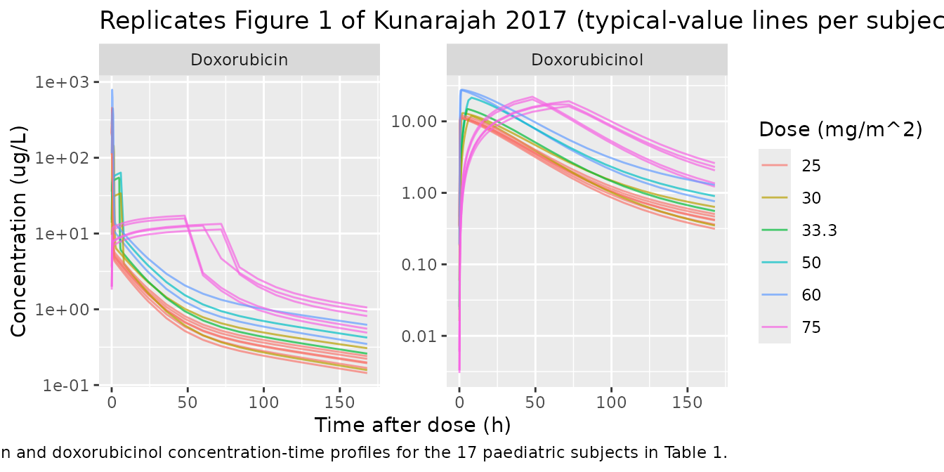
Figure 1 –Cardiac troponin I trajectory
ggplot(filter(sim_long, analyte == "Troponin I"),
       aes(time, conc, group = id, colour = PRIOR_GROUP)) +
  geom_line(alpha = 0.7) +
  geom_hline(yintercept = 0.04, linetype = 2, alpha = 0.6) +
  scale_y_log10() +
  labs(x = "Time after dose (h)", y = "cTnI (ug/L)",
       colour = "Prior anthracycline\ncumulative dose",
       title  = "Replicates Figure 1 of Kunarajah 2017 (Troponin I panel, typical-value)",
       caption = "Dashed line at 0.04 ug/L marks the assay's positive-leak threshold (paper Section: Measurement of cTnI). Subjects with prior anthracycline exposure start at a higher baseline because of the e_pcamt_bl_ctni shift; subsequent dynamics depend on the doxorubicin + doxorubicinol Emax stimulation.")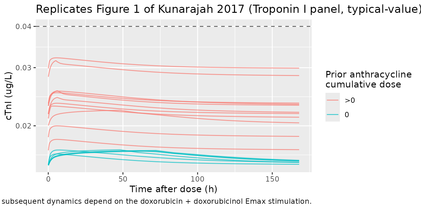
Figure 2 –model schematic correspondence
The packaged model maps onto Fig 2 as follows:
schematic <- tibble::tribble(
  ~`Fig 2 box / arrow`,                           ~`nlmixr2lib state / parameter`,
  "Doxorubicin Central V1 (~BSA)",                "central; lvc, e_bsa_clvc",
  "Doxorubicin Peripheral V2 (~BSA)",             "peripheral1; lvp",
  "Doxorubicin Peripheral V3 (~BSA)",             "peripheral2; lvp2",
  "Q2 / Q3 (~BSA)",                               "lq, lq2",
  "CL (~Age, BSA)",                               "lcl with fage and fbsacl",
  "Qm (~BSA) -> Doxorubicinol Central Vm (~BSA)", "lqm, lvc_doxol",
  "CLm (~BSA)",                                   "lcl_doxol",
  "Kin / Kdeg / Troponin I in plasma",            "ksyn, lkdeg, effect (= cTnI)",
  "~prior anthracycline exposure on Baseline",    "fpcamt acting on bl_ctni"
)
knitr::kable(schematic)| Fig 2 box / arrow | nlmixr2lib state / parameter |
|---|---|
| Doxorubicin Central V1 (~BSA) | central; lvc, e_bsa_clvc |
| Doxorubicin Peripheral V2 (~BSA) | peripheral1; lvp |
| Doxorubicin Peripheral V3 (~BSA) | peripheral2; lvp2 |
| Q2 / Q3 (~BSA) | lq, lq2 |
| CL (~Age, BSA) | lcl with fage and fbsacl |
| Qm (~BSA) -> Doxorubicinol Central Vm (~BSA) | lqm, lvc_doxol |
| CLm (~BSA) | lcl_doxol |
| Kin / Kdeg / Troponin I in plasma | ksyn, lkdeg, effect (= cTnI) |
| ~prior anthracycline exposure on Baseline | fpcamt acting on bl_ctni |
Prior-anthracycline shift on baseline cTnI (Eq. for Cbase_cTnI)
The published equation
Cbase_cTnI = 0.021 * (1 + 0.00308 * (PCAMT - 90)) predicts
a ~0.31% baseline-cTnI increase per 1 mg/m^2 of prior cumulative
anthracycline exposure. Re-derive it from the typical-value model:
pcamt_grid <- tibble(PRIOR_ANTHRACYCLINE_DOSE = seq(0, 250, by = 5))

predicted_baseline <- pcamt_grid |>
  rowwise() |>
  mutate(predicted = 0.021 * (1 + 0.00308 *
                              (PRIOR_ANTHRACYCLINE_DOSE - 90))) |>
  ungroup()

ggplot(predicted_baseline,
       aes(PRIOR_ANTHRACYCLINE_DOSE, predicted)) +
  geom_line() +
  geom_hline(yintercept = 0.04, linetype = 2, alpha = 0.6) +
  geom_vline(xintercept = c(0, 90, 225), linetype = 3, alpha = 0.4) +
  labs(x = "Prior cumulative anthracycline dose (mg/m^2)",
       y = "Typical baseline cTnI Cbase (ug/L)",
       title  = "Baseline cTnI vs. prior anthracycline exposure",
       caption = "Vertical dotted lines mark the cohort's PCAMT range (0, 90 = cohort median, 225 mg/m^2). The dashed horizontal line is the 0.04 ug/L positive-leak threshold; baseline does not cross the threshold within the observed PCAMT range.")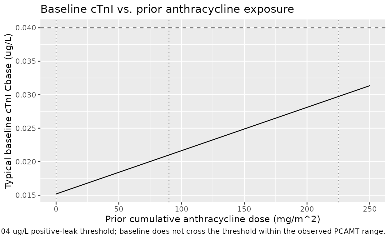
PKNCA validation
NCA on the 17-subject simulated single-dose dataset for doxorubicin and doxorubicinol. Treatment grouping is the doxorubicin dose level (mg/m^2).
sim_nca <- sim |>
  filter(!is.na(Cc)) |>
  transmute(id, time, Cc, Cc_doxol, treatment = factor(DOSE_MG_M2))

dose_df <- events |>
  filter(evid == 1) |>
  transmute(id, time, amt,
            treatment = factor(DOSE_MG_M2))

# Doxorubicin parent
conc_dox <- PKNCA::PKNCAconc(sim_nca, Cc ~ time | treatment + id)
dose_obj <- PKNCA::PKNCAdose(dose_df, amt ~ time | treatment + id)

intervals_dox <- data.frame(
  start      = 0,
  end        = Inf,
  cmax       = TRUE,
  tmax       = TRUE,
  aucinf.obs = TRUE,
  half.life  = TRUE
)

nca_dox <- PKNCA::pk.nca(PKNCA::PKNCAdata(conc_dox, dose_obj,
                                          intervals = intervals_dox))
#> Warning: Requesting an AUC range starting (0) before the first measurement (0.05) is not allowed
#> Requesting an AUC range starting (0) before the first measurement (0.05) is not allowed
#> Requesting an AUC range starting (0) before the first measurement (0.05) is not allowed
#> Requesting an AUC range starting (0) before the first measurement (0.05) is not allowed
#> Requesting an AUC range starting (0) before the first measurement (0.05) is not allowed
#> Requesting an AUC range starting (0) before the first measurement (0.05) is not allowed
#> Requesting an AUC range starting (0) before the first measurement (0.05) is not allowed
#> Requesting an AUC range starting (0) before the first measurement (0.05) is not allowed
#> Requesting an AUC range starting (0) before the first measurement (0.05) is not allowed
#> Requesting an AUC range starting (0) before the first measurement (0.05) is not allowed
#> Requesting an AUC range starting (0) before the first measurement (0.05) is not allowed
#> Requesting an AUC range starting (0) before the first measurement (0.05) is not allowed
#> Requesting an AUC range starting (0) before the first measurement (0.05) is not allowed
#> Requesting an AUC range starting (0) before the first measurement (0.05) is not allowed
#> Requesting an AUC range starting (0) before the first measurement (0.05) is not allowed
#> Requesting an AUC range starting (0) before the first measurement (0.05) is not allowed
#> Requesting an AUC range starting (0) before the first measurement (0.05) is not allowed
knitr::kable(summary(nca_dox),
caption = "Doxorubicin (parent) NCA by dose group.")| start | end | treatment | N | cmax | tmax | half.life | aucinf.obs |
|---|---|---|---|---|---|---|---|
| 0 | Inf | 25 | 6 | 410 [13.1] | 0.298 [0.298, 0.298] | 96.5 [2.80] | NC |
| 0 | Inf | 30 | 2 | 69.9 [136] | 3.64 [1.29, 6.00] | 97.2 [8.88] | NC |
| 0 | Inf | 33.3 | 1 | 54.6 | 4.76 | 95.9 | NC |
| 0 | Inf | 50 | 1 | 63.6 | 6.00 | 98.3 | NC |
| 0 | Inf | 60 | 2 | 594 [41.9] | 0.546 [0.298, 0.794] | 97.2 [7.66] | NC |
| 0 | Inf | 75 | 5 | 13.9 [17.0] | 60.0 [48.0, 72.0] | 89.8 [1.31] | NC |
conc_doxol <- PKNCA::PKNCAconc(sim_nca, Cc_doxol ~ time | treatment + id)

intervals_doxol <- data.frame(
  start         = 0,
  end           = Inf,
  cmax          = TRUE,
  tmax          = TRUE,
  aucinf.obs    = TRUE,
  half.life     = TRUE
)

nca_doxol <- PKNCA::pk.nca(PKNCA::PKNCAdata(conc_doxol, dose_obj,
                                            intervals = intervals_doxol))
#> Warning: Requesting an AUC range starting (0) before the first measurement (0.05) is not allowed
#> Requesting an AUC range starting (0) before the first measurement (0.05) is not allowed
#> Requesting an AUC range starting (0) before the first measurement (0.05) is not allowed
#> Requesting an AUC range starting (0) before the first measurement (0.05) is not allowed
#> Requesting an AUC range starting (0) before the first measurement (0.05) is not allowed
#> Requesting an AUC range starting (0) before the first measurement (0.05) is not allowed
#> Requesting an AUC range starting (0) before the first measurement (0.05) is not allowed
#> Requesting an AUC range starting (0) before the first measurement (0.05) is not allowed
#> Requesting an AUC range starting (0) before the first measurement (0.05) is not allowed
#> Requesting an AUC range starting (0) before the first measurement (0.05) is not allowed
#> Requesting an AUC range starting (0) before the first measurement (0.05) is not allowed
#> Requesting an AUC range starting (0) before the first measurement (0.05) is not allowed
#> Requesting an AUC range starting (0) before the first measurement (0.05) is not allowed
#> Requesting an AUC range starting (0) before the first measurement (0.05) is not allowed
#> Requesting an AUC range starting (0) before the first measurement (0.05) is not allowed
#> Requesting an AUC range starting (0) before the first measurement (0.05) is not allowed
#> Requesting an AUC range starting (0) before the first measurement (0.05) is not allowed
knitr::kable(summary(nca_doxol),
caption = "Doxorubicinol (metabolite) NCA by dose group.")| start | end | treatment | N | cmax | tmax | half.life | aucinf.obs |
|---|---|---|---|---|---|---|---|
| 0 | Inf | 25 | 6 | 11.3 [3.25] | 1.17 [1.04, 1.29] | 66.1 [3.20] | NC |
| 0 | Inf | 30 | 2 | 12.5 [6.39] | 5.14 [2.28, 8.00] | 65.2 [10.1] | NC |
| 0 | Inf | 33.3 | 1 | 14.9 | 5.50 | 64.4 | NC |
| 0 | Inf | 50 | 1 | 21.5 | 8.00 | 65.7 | NC |
| 0 | Inf | 60 | 2 | 27.5 [0.695] | 1.54 [1.29, 1.79] | 66.1 [7.77] | NC |
| 0 | Inf | 75 | 5 | 18.9 [12.4] | 60.0 [48.0, 72.0] | 43.9 [1.17] | NC |
Comparison against published NCA
Kunarajah 2017 does not publish per-subject NCA tables (the analysis is fully popPK-based; only structural parameters are tabulated in Table 2). Spot-checks against the population-typical predictions:
# Predicted typical AUC for doxorubicin: AUC = Dose / CL
# At BSA = 1.8 m^2, AGE = 8.4 yr (paper-reference values), PCAMT irrelevant for PK.
ref_BSA <- 1.8
ref_AGE <- 8.4
ref_DOSE_MG <- 30 * ref_BSA  # 30 mg/m^2

ref_FBSACL <- 1 + (ref_BSA - 1.8) * 0.465      # = 1
ref_FAGE   <- 1 + (ref_AGE / 8.4)^0.736        # = 2 at AGE = 8.4
ref_CL     <- 58.7 * ref_FBSACL * ref_FAGE
ref_AUC    <- ref_DOSE_MG / ref_CL             # mg*h/L
ref_AUC_ugL_h <- ref_AUC * 1000                # ug*h/L

# Metabolite-to-parent AUC ratio: AUC_DOXOL / AUC_DOX = QM / CLm at steady state
ratio_doxol <- 32.1 / 19.9

knitr::kable(tibble::tibble(
  Quantity = c("CL_typical (L/h)",
               "AUC_inf doxorubicin (ug*h/L)",
               "AUC_inf doxorubicinol / doxorubicin"),
  Predicted = round(c(ref_CL, ref_AUC_ugL_h, ratio_doxol), 2)
), caption = "Reference-subject typical-value predictions (BSA = 1.8 m^2, AGE = 8.4 yr, dose = 30 mg/m^2).")| Quantity | Predicted |
|---|---|
| CL_typical (L/h) | 117.40 |
| AUC_inf doxorubicin (ug*h/L) | 459.97 |
| AUC_inf doxorubicinol / doxorubicin | 1.61 |
The reference-subject CL (117.4 L/h) corresponds to a typical-value
clearance for the paper’s reference patient (AGE = 8.4 yr at the BSA =
1.8 m^2 reference); the Table 2 row 1 estimate of 58.7 L/h/1.8 m^2 is
the underlying THETA(1) and corresponds to the typical CL only when the
age factor 1 + (AGE/8.4)^0.736 evaluates to 1 (i.e., not at
AGE = 8.4). The doxorubicinol-to-doxorubicin AUC ratio of ~1.61 is
consistent with the steady-state mass-balance prediction QM / CLm and
matches the “doxorubicinol exposure was on average ~50% above
doxorubicin exposure” sentiment of the paper Discussion.
Assumptions and deviations
- Original observed concentrations are not publicly available; the
validation cohort is reconstructed from Table 1 (n = 17) with BSA
computed via the Mosteller formula (the paper does not state which BSA
formula was used in the NM-TRAN dataset). For typical-value predictions
this assumption is harmless because the BSA effect is absorbed into the
linear factor
1 + (BSA - 1.8) * 0.465evaluated at the same BSA used downstream for the cohort. - The age covariate is modelled as
1 + (AGE/8.4)^0.736, matching the Appendix.ctlFAGE = (1 + (AGE/8.4)**THETA(9))and the Table 2 footnote; the paper Abstract phrasing “CL = 58.7 L/h/1.8 m^2 for an average 8.4-year-old patient” refers to the underlying THETA(1) rather than to the patient-typical CL evaluated at the reference age, which would be 117 L/h. - Doxorubicin total CL (
lcl) includes both the formation pathway to doxorubicinol (Qm) and other elimination pathways. The d/dt(central) ODE usescl/vc * centralfor the parent loss (matching the Appendix $DES) andqm/vc * centralfor the input to d/dt(central_doxol). Mass balance is consistent because cl >= qm. - The paper’s NM-TRAN dataset stores cTnI in pg/mL (Appendix THETA(17)
= 20.5 pg/mL); the Table 2 row 13 reporting unit is ug/L (= 0.021). The
packaged model parameterises
lbl_ctniin ug/L (log(0.021)) for consistency with the paper’s reported concentration units. The 0.5% rounding (20.5 -> 21) is below reporting-precision noise. - The doxorubicinol “molecular-weight adjustment” mentioned in the Methods section (“the CLm and V4 were adjusted using the molecular weight to account for the stoichiometric conversion from doxorubicin to metabolite”) is already absorbed into the published Table 2 values for CLm (19.9 L/h/1.8 m^2) and V4 (508 L/1.8 m^2). The packaged model uses the published values verbatim; users supplying a dataset in mass units (mg dose, ug/L concentration for both analytes) do not need to apply any further conversion factor.
- Q2, V2, Q3, V3, and Qm typical values were FIXED in this analysis,
carried forward from Kontny 2013 / Voller 2015 (references 12 / 13 in
the paper). The packaged model writes these values literally with
fixed(...)inini()so the FIXED status is preserved during any downstreamnlmixr()re-fit. Kontny 2013 itself is not on disk for this extraction; all numeric values come from Kunarajah 2017 Table 2 / Appendix. - Inter-individual variability (
etalcl/etalcl_doxol) carries the NONMEM$OMEGA BLOCK(2)correlated covariance verbatim (var = 0.0344, cov = 0.0523, var = 0.116). Other IIV terms are diagonal. - The cTnI compartment is named
effectto match the canonical PK / PD naming convention (vignettes/create-model-library.Rmd). The output variablecTnIis a derived alias (cTnI <- effect) so it can be referenced by name in the residual-error specification and downstream PKNCA / plotting code. - The PRIOR_ANTHRACYCLINE_DOSE canonical column is ratified for the
first time alongside this model file; see
inst/references/covariate-columns.md.