Shikimic acid PK and immune-enhancing PD in growing pigs (Mo 2024)

Model and source

Shikimic acid (SA) is a trihydroxycyclohexene carboxylic acid used as a food preservative and as the synthetic precursor of oseltamivir. Mo 2024 is the first report of its pharmacokinetics in pigs. Six growing pigs received SA in a two-period, two-sequence crossover: 50 mg/kg by gavage in one period and 2 mg/kg into the marginal ear vein in the other, separated by a 7-day washout. Plasma SA was measured by HPLC-MS/MS, and complement C3 and C4 and immunoglobulin G, A and M were measured by ELISA in the same samples.

The authors selected different structural models for the two routes by AIC (Section 2.6, supplementary Table S2) and fitted each pig individually in Phoenix WinNonlin, so the paper contributes two independent model files:

sa_models <- c(
  "Mo_2024_shikimicAcid_pig_iv",    # 2-compartment IV disposition + sigmoid-Emax PD
  "Mo_2024_shikimicAcid_pig_oral"   # 1-compartment first-order absorption
)

# Parse each model once; the parsed object is what exposes the file-level
# metadata (reference, description, population) as well as being solvable.
mod_iv   <- rxode2::rxode(readModelDb(sa_models[1]))
mod_oral <- rxode2::rxode(readModelDb(sa_models[2]))

The immune-response (PD) layer belongs to the intravenous model only: Mo 2024 fitted sigmoid-Emax models to the intravenous group because the intragastric effect-versus-concentration curves were not monotonic (Section 4, Figures S4 and S5).

• Citation: Mo K, Shen Y, Su D, Lv L, Du J, Ding H, Huang X (2024). Pharmacokinetic-Pharmacodynamic Modeling of the Immune-Enhancing Effect of Shikimic Acid in Growing Pigs. J Agric Food Chem 72:26224-26235. doi:10.1021/acs.jafc.4c09250
• Article: J Agric Food Chem 2024;72:26224-26235

sa_parsed <- stats::setNames(list(mod_iv, mod_oral), sa_models)
for (m in sa_models) {
  cat(m, "\n", sep = "")
  cat(strwrap(sa_parsed[[m]]$description, 76), sep = "\n")
  cat("\n\n")
}
#> Mo_2024_shikimicAcid_pig_iv
#> Preclinical (pig). Two-compartment intravenous pharmacokinetic model for
#> shikimic acid (SA) in growing Landrace x Large White pigs, coupled to five
#> direct-effect sigmoid-Emax pharmacodynamic models for the immune-enhancing
#> effect of SA on plasma complement and immunoglobulin (Mo 2024). SA was
#> given as a single 2 mg/kg injection into the marginal ear vein. The paper
#> reports the intravenous disposition as the biexponential C =
#> A*exp(-alpha*t) + B*exp(-beta*t) (Table 10); the central volume, clearance,
#> intercompartmental clearance and peripheral volume carried here are derived
#> from the mean A, alpha, B and beta and reproduce that equation. The
#> pharmacodynamic layer links the SA plasma concentration to the absolute
#> change from the predose (0 h) level of complement C3 and C4 and of
#> immunoglobulin G, A and M through E = Emax * C^gamma / (EC50^gamma +
#> C^gamma) (eq 2; parameters in Table 11), with no effect compartment because
#> Mo 2024 found no hysteresis between concentration and effect. All
#> disposition and effect states are expressed per kg body weight (volumes in
#> mL/kg, clearances in mL/h/kg, amounts in ng/kg). Mo 2024 fitted each pig
#> individually in Phoenix WinNonlin and reported only the mean and SD of the
#> individual estimates, so no between-subject variability or residual-error
#> model is available; every parameter is fixed at the published mean and the
#> residual SDs are fixed at zero. The companion intragastric model is
#> modellib('Mo_2024_shikimicAcid_pig_oral').
#> 
#> 
#> Mo_2024_shikimicAcid_pig_oral
#> Preclinical (pig). One-compartment first-order-absorption pharmacokinetic
#> model for shikimic acid (SA) in growing Landrace x Large White pigs after a
#> single 50 mg/kg intragastric (gavage) dose (Mo 2024). Mo 2024 selected this
#> structure over a two-compartment and over lag-time alternatives by AIC
#> (Section 2.6, supplementary Table S2) and describes the profile as C =
#> M*(exp(-ke*t) - exp(-ka*t)); the absorption and elimination rate constants
#> carried here are back-calculated from the reported absorption and
#> elimination half-lives, and the volume from the reported apparent
#> clearance. Because only the extravascular route is observed, clearance and
#> volume are apparent (Cl/F and V/F); the absolute bioavailability of SA in
#> these pigs was 21.68 percent. All states are expressed per kg body weight
#> (volume in mL/kg, clearance in mL/h/kg, amounts in ng/kg). Two of the six
#> pigs showed a double peak that this single-depot model does not reproduce.
#> Mo 2024 fitted each pig individually in Phoenix WinNonlin and reported only
#> the mean and SD of the individual estimates, so no between-subject
#> variability or residual-error model is available; every parameter is fixed
#> at the published mean and the residual SD is fixed at zero. No
#> pharmacodynamic model accompanies this route - Mo 2024 fitted the
#> sigmoid-Emax immune-response models to the intravenous group only; see
#> modellib('Mo_2024_shikimicAcid_pig_iv').

Population

Six growing pigs (Landrace x Large White, approximately 90 days old, both sexes) of comparable health status and genetic background were randomised to sequence A (n = 3) or sequence B (n = 3) after a 7-day acclimatisation (Mo 2024 Section 2.2, Table 1). Every pig contributed both an intragastric and an intravenous profile, so the same six animals support both model files. Plasma was drawn from the anterior vena cava predose and at 0.083 (intravenous only), 0.25, 0.5, 0.75, 1, 1.5, 2, 3, 4, 6, 8, 12 and 24 h; complement and immunoglobulin were assayed at 0, 0.5, 1, 1.5, 3, 6 and 12 h (Sections 2.3 and 2.5).

Body weights are reported only in supplementary Table S1, which is not part of the open-access record; the paper states that weight did not differ between the two periods (P = 0.320). Because every parameter in both models is expressed per kg body weight, no weight covariate is needed to simulate them.

str(mod_iv$population)
#> List of 9
#>  $ species      : chr "pig (Landrace x Large White)"
#>  $ n_subjects   : num 6
#>  $ n_studies    : num 1
#>  $ age_median   : chr "approximately 90 days"
#>  $ sex          : chr "male and female"
#>  $ disease_state: chr "healthy growing pigs"
#>  $ dose_range   : chr "shikimic acid 2 mg/kg as a single marginal-ear-vein injection"
#>  $ regions      : chr "China"
#>  $ notes        : chr "Mo 2024 Section 2.2 and Table 1: six growing pigs of comparable health status and genetic background, approxima"| __truncated__

Source trace

Both model files carry the origin of each value as an in-file comment next to its ini() entry. The table below collects them.

Equation / parameter	Value	Source location
Mo_2024_shikimicAcid_pig_iv
IV disposition equation C = A*exp(-alpha*t) + B*exp(-beta*t)	n/a	Section 3.2, second paragraph
lvc (central volume)	244.81 mL/kg	derived: Dose/(A + B) from Table 10 means
lcl (clearance)	229.14 mL/h/kg	derived: k10*vc from Table 10 means
lq (intercompartmental clearance)	115.23 mL/h/kg	derived: k12*vc from Table 10 means
lvp (peripheral volume)	300.58 mL/kg	derived: q/k21 from Table 10 means
PD equation E = Emax*C^gamma/(EC50^gamma + C^gamma)	n/a	eq 2, Section 2.6
lemax_c3 / lec50_c3 / lhill_c3	352.95 ug/mL / 700.45 ng/mL / 3.77	Table 11, row C3
lemax_c4 / lec50_c4 / lhill_c4	0.064 ug/mL / 836.61 ng/mL / 3.89	Table 11, row C4
lemax_igg / lec50_igg / lhill_igg	9801.86 ug/mL / 514.22 ng/mL / 5.15	Table 11, row IgG
lemax_iga / lec50_iga / lhill_iga	469.30 ug/mL / 561.88 ng/mL / 6.97	Table 11, row IgA
lemax_igm / lec50_igm / lhill_igm	1252.05 ug/mL / 686.24 ng/mL / 3.75	Table 11, row IgM
addSd, addSd_dC3 … addSd_dIgM	0 (fixed)	not reported; see Errata
Mo_2024_shikimicAcid_pig_oral
Absorption equation C = M*(exp(-ke*t) - exp(-ka*t))	n/a	Section 3.2, first paragraph (sign corrected; see Errata)
lka	0.815467 /h	derived: ln(2)/0.85 h from Table 9 t1/2ka
lcl (apparent Cl/F)	1086.52 mL/h/kg	Table 9, Cl_F
lvc (apparent V/F)	2837.21 mL/kg	derived: Cl_F/(ln(2)/1.81 h) from Table 9
addSd	0 (fixed)	not reported; see Errata

Reconstructing the disposition parameters from Table 10

Mo 2024 tabulates the intravenous fit as the biexponential coefficients and exponents rather than as volumes and clearances, so the packaged parameters are a transformation of Table 10. The chunk below performs that transformation and solves it back, confirming that the packaged values regenerate Table 10.

A <- 7227.76; B <- 941.91; alpha <- 1.56; beta <- 0.23   # Table 10, mean column
dose_iv <- 2e6                                           # 2 mg/kg expressed as ng/kg

vc  <- dose_iv / (A + B)
k21 <- (A * beta + B * alpha) / (A + B)
k10 <- alpha * beta / k21
k12 <- alpha + beta - k21 - k10
cl  <- k10 * vc
q   <- k12 * vc
vp  <- q / k21

# Round as packaged, then solve the rounded values back to a biexponential.
vcr <- round(vc, 2); clr <- round(cl, 2); qr <- round(q, 2); vpr <- round(vp, 2)
K10 <- clr / vcr; K12 <- qr / vcr; K21 <- qr / vpr
s <- K10 + K12 + K21; p <- K10 * K21
Al <- (s + sqrt(s^2 - 4 * p)) / 2
Be <- (s - sqrt(s^2 - 4 * p)) / 2

data.frame(
  quantity  = c("A (ng/mL)", "alpha (1/h)", "B (ng/mL)", "beta (1/h)"),
  published = c(A, alpha, B, beta),
  recovered = round(c(dose_iv / vcr * (Al - K21) / (Al - Be), Al,
                      dose_iv / vcr * (K21 - Be) / (Al - Be), Be), 4)
) |>
  dplyr::rename("Table 10 quantity" = quantity,
                "Published" = published,
                "Recovered from packaged model" = recovered) |>
  knitr::kable(caption = "The packaged vc/cl/q/vp regenerate Table 10 to rounding.")

The packaged vc/cl/q/vp regenerate Table 10 to rounding.

Table 10 quantity	Published	Recovered from packaged model
A (ng/mL)	7227.76	7227.6538
alpha (1/h)	1.56	1.5600
B (ng/mL)	941.91	941.9471
beta (1/h)	0.23	0.2300

Mo 2024 also tabulates secondary parameters computed independently of the biexponential, which act as an external check on the transformation:

data.frame(
  parameter = c("Cl (mL/h/kg)", "Vss (mL/kg)", "peripheral volume (mL/kg)"),
  published = c(233.20, 574.10, 323.11),
  derived   = round(c(cl, vc + vp, vp), 2)
) |>
  dplyr::mutate("Difference (%)" = round(100 * (derived - published) / published, 1)) |>
  dplyr::rename("Parameter" = parameter,
                "Mo 2024 Table 10" = published,
                "Derived here" = derived) |>
  knitr::kable(caption = paste(
    "Secondary-parameter cross-check. Differences arise because Table 10 reports",
    "the mean of six individually derived values whereas the packaged model",
    "transforms the mean biexponential; the two are not algebraically identical."
  ))

Secondary-parameter cross-check. Differences arise because Table 10 reports the mean of six individually derived values whereas the packaged model transforms the mean biexponential; the two are not algebraically identical.

Parameter	Mo 2024 Table 10	Derived here	Difference (%)
Cl (mL/h/kg)	233.20	229.14	-1.7
Vss (mL/kg)	574.10	545.39	-5.0
peripheral volume (mL/kg)	323.11	300.58	-7.0

The V_Z column of Table 10 is the peripheral volume

Table 10 labels a column V_Z (mean 323.11 mL/kg) and the abbreviation list glosses it as “the apparent volume of distribution”. Taken as the terminal-phase volume it is irreconcilable with the rest of the table: Cl/beta runs from 660 to 1913 mL/kg across the six pigs (mean 1115), i.e. 2.3 to 4.9 times the tabulated V_Z of the same animal. The column is in fact the peripheral volume, because Vss - V_Z equals Dose/(A + B) – the central volume – for every one of the six pigs:

pigs <- data.frame(
  A    = c(5520.89, 6305.87, 7713.37, 6992.87, 7849.21, 8984.33),
  B    = c(1115.22,  357.49, 1181.81,  590.59, 1658.52,  747.84),
  Vss  = c( 794.73,  777.21,  486.09,  581.23,  417.74,  387.64),
  Vz   = c( 493.34,  477.06,  261.25,  317.50,  207.38,  182.13),
  Cl   = c( 125.28,  382.68,  271.04,  174.31,  250.80,  195.07),
  beta = c(   0.11,    0.20,    0.32,    0.14,    0.38,    0.22),
  thalf_beta = c(6.41, 3.42, 2.16, 5.01, 1.84, 3.11)
)
pigs |>
  dplyr::transmute(
    pig            = seq_len(dplyr::n()),
    `Dose/(A+B)`   = round(2e6 / (A + B), 2),
    `Vss - V_Z`    = round(Vss - Vz, 2),
    `Cl/beta`      = round(Cl / beta, 0)
  ) |>
  knitr::kable(caption = paste(
    "Vss - V_Z reproduces the central volume Dose/(A+B) to within 0.01 mL/kg for",
    "all six pigs, whereas the terminal-phase volume Cl/beta does not match V_Z",
    "at all."
  ))

Vss - V_Z reproduces the central volume Dose/(A+B) to within 0.01 mL/kg for all six pigs, whereas the terminal-phase volume Cl/beta does not match V_Z at all.

pig	Dose/(A+B)	Vss - V_Z	Cl/beta
1	301.38	301.39	1139
2	300.15	300.15	1913
3	224.84	224.84	847
4	263.73	263.73	1245
5	210.36	210.36	660
6	205.50	205.51	887

stopifnot(max(abs(2e6 / (pigs$A + pigs$B) - (pigs$Vss - pigs$Vz))) < 0.02)

The packaged lvp therefore corresponds to that column, and no terminal-phase volume is carried.

Virtual cohort

Mo 2024 fitted each animal separately and reported only the mean and SD of the individual estimates, so neither model carries between-subject variability or a residual-error model (see Errata). Both simulations below are therefore deterministic single typical-animal profiles at the studied dose levels, on the paper’s own sampling schedule augmented with a dense grid for plotting.

obs_iv   <- c(0, 0.083, 0.25, 0.5, 0.75, 1, 1.5, 2, 3, 4, 6, 8, 12)
obs_oral <- c(0, 0.25, 0.5, 0.75, 1, 1.5, 2, 3, 4, 6, 8, 12, 24)
obs_pd   <- c(0, 0.5, 1, 1.5, 3, 6, 12)

grid_iv   <- sort(unique(c(obs_iv,   obs_pd, seq(0, 12, length.out = 241))))
# The intragastric grid is refined around the absorption peak so that the NCA
# T_max reflects the model rather than the spacing of the observation grid.
grid_oral <- sort(unique(c(obs_oral, seq(0, 24, length.out = 241),
                          seq(1, 2.5, by = 0.01))))

# Intravenous: six algebraic endpoints (Cc plus five immune markers), so
# observation rows carry dvid = 1 and no cmt. rxode2 returns every algebraic
# observable as a column regardless of which endpoint the row names.
ev_iv <- as.data.frame(
  rxode2::et(amt = dose_iv, cmt = "central") |>
    rxode2::et(grid_iv)
)
ev_iv$dvid <- ifelse(ev_iv$evid == 0, 1L, NA_integer_)
ev_iv$id <- 1L

# Intragastric: single endpoint, so observations sit on the central ODE state.
dose_oral <- 5e7   # 50 mg/kg expressed as ng/kg
ev_oral <- as.data.frame(
  rxode2::et(amt = dose_oral, cmt = "depot") |>
    rxode2::et(grid_oral, cmt = "central")
)
ev_oral$id <- 1L

c(iv_rows = nrow(ev_iv), oral_rows = nrow(ev_oral))
#>   iv_rows oral_rows 
#>       243       383

Simulation

sim_iv <- rxode2::rxSolve(
  mod_iv, ev_iv,
  returnType = "data.frame", addDosing = FALSE
)
sim_oral <- rxode2::rxSolve(
  mod_oral, ev_oral,
  returnType = "data.frame", addDosing = FALSE
)

stopifnot(nrow(sim_iv) > 0, nrow(sim_oral) > 0)
stopifnot(all(c("Cc", "dC3", "dC4", "dIgG", "dIgA", "dIgM") %in% names(sim_iv)))
stopifnot(!anyNA(sim_iv$Cc), !anyNA(sim_oral$Cc))

Replicate published figures

Figure 3B – intravenous concentration-time profile

The simulated curve is overlaid on the paper’s own analytic solution C = A*exp(-alpha*t) + B*exp(-beta*t) evaluated at the Table 10 means, and on the observed mean C_max.

# Evaluated at the solver's own output times so the overlay and the numeric
# check below are aligned by construction.
analytic_iv <- data.frame(time = sim_iv$time) |>
  dplyr::mutate(Cc = A * exp(-alpha * time) + B * exp(-beta * time))

ggplot(sim_iv, aes(time, Cc)) +
  geom_line(linewidth = 1) +
  geom_line(data = analytic_iv, aes(time, Cc),
            colour = "firebrick", linetype = "22", linewidth = 0.9) +
  geom_point(data = data.frame(time = 0, Cc = 8169.67),
             aes(time, Cc), colour = "firebrick", size = 2.5) +
  geom_hline(yintercept = 20, linetype = "dotted", colour = "grey40") +
  scale_y_log10() +
  labs(
    x = "Time (h)", y = "Shikimic acid (ng/mL, log scale)",
    subtitle = paste("Black: packaged model. Red dashed: Mo 2024 analytic biexponential.",
                     "\nRed point: reported mean C_max. Dotted line: LOQ 20 ng/mL.")
  ) +
  theme_bw()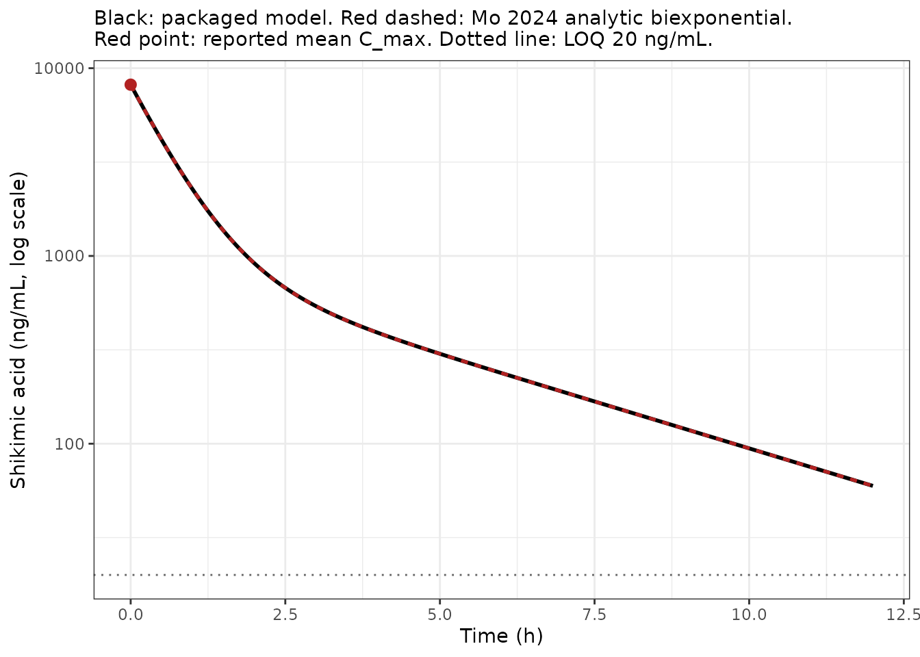

Replicates Figure 3B of Mo 2024 (intravenous, 2 mg/kg).

max_rel_err <- max(abs(sim_iv$Cc - analytic_iv$Cc) / analytic_iv$Cc)
cat(sprintf("Largest relative deviation from the published equation: %.4f%%\n",
            100 * max_rel_err))
#> Largest relative deviation from the published equation: 0.0059%
stopifnot(max_rel_err < 0.01)

Figure 3A – intragastric concentration-time profile

ggplot(sim_oral, aes(time, Cc)) +
  geom_line(linewidth = 1) +
  geom_point(data = data.frame(time = 1.78, Cc = 10823.44),
             aes(time, Cc), colour = "firebrick", size = 2.5) +
  geom_errorbar(
    data = data.frame(time = 1.78, lo = 10823.44 - 4934.04, hi = 10823.44 + 4934.04),
    aes(x = time, ymin = lo, ymax = hi), inherit.aes = FALSE,
    width = 0.4, colour = "firebrick"
  ) +
  labs(
    x = "Time (h)", y = "Shikimic acid (ng/mL)",
    subtitle = paste("Black: packaged model. Red: reported mean C_max at mean T_max",
                     "(+/- SD of C_max), Table 9.")
  ) +
  theme_bw()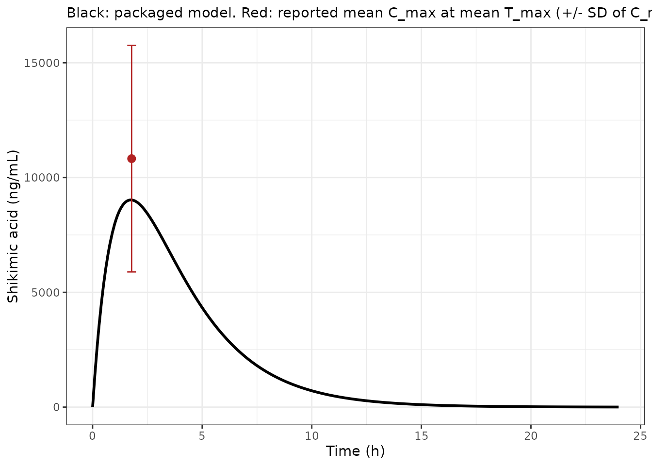

Replicates Figure 3A of Mo 2024 (intragastric, 50 mg/kg).

Figure 5 – immune-marker time courses after intravenous dosing

The PD layer predicts the absolute change from the predose level, which is what Mo 2024’s eq 2 models. Figure 5 plots absolute concentrations; the paper’s baselines are not tabulated, so the change is plotted directly.

One difference from Figure 5 is structural rather than a discrepancy. In the model, t = 0 is the instant after the bolus, where the concentration is already at C_max; because eq 2 is a direct-effect model with no effect compartment, the predicted change is therefore already near E_max at t = 0. In the paper, the 0 h ELISA sample is the predose baseline, against which the change is defined as zero, and the first post-dose measurement is at 0.5 h. The model consequently cannot show the 0-to-0.5 h rise that Figure 5 displays: a direct-effect model driven by a bolus has no mechanism to delay the onset. Mo 2024’s own finding of no hysteresis is what licenses that structure. The two testable features among the post-dose samples are that the effect is maximal at the earliest one (0.5 h) and has returned to the predose level by 12 h.

pd_long <- sim_iv |>
  dplyr::select(time, dC3, dC4, dIgG, dIgA, dIgM) |>
  tidyr::pivot_longer(-time, names_to = "marker", values_to = "delta") |>
  dplyr::mutate(marker = factor(
    marker,
    levels = c("dC3", "dC4", "dIgG", "dIgA", "dIgM"),
    labels = c("C3", "C4", "IgG", "IgA", "IgM")
  ))

ggplot(pd_long, aes(time, delta)) +
  geom_line(linewidth = 1) +
  geom_vline(xintercept = c(0.5, 12), linetype = "dotted", colour = "grey40") +
  facet_wrap(~marker, scales = "free_y") +
  labs(x = "Time (h)", y = "Change from predose (ug/mL)",
       subtitle = "Dotted lines: the 0.5 h peak and the 12 h return to predose reported by Mo 2024.") +
  theme_bw()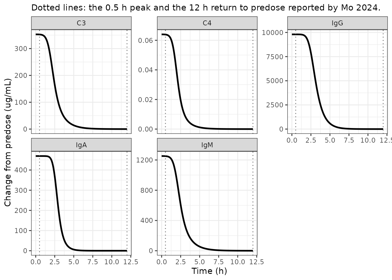

Replicates the time-course shape of Figure 5 of Mo 2024 (intravenous).

pd_at <- function(t) {
  sim_iv[which.min(abs(sim_iv$time - t)), c("dC3", "dC4", "dIgG", "dIgA", "dIgM")]
}
emax_pub <- c(dC3 = 352.95, dC4 = 0.064, dIgG = 9801.86, dIgA = 469.30, dIgM = 1252.05)

data.frame(
  marker      = names(emax_pub),
  emax        = unname(emax_pub),
  at_0.5h     = as.numeric(pd_at(0.5)),
  at_12h      = as.numeric(pd_at(12))
) |>
  dplyr::mutate(
    `Percent of Emax at 0.5 h` = round(100 * at_0.5h / emax, 1),
    `Percent of Emax at 12 h`  = round(100 * at_12h  / emax, 2)
  ) |>
  dplyr::select(-at_0.5h, -at_12h) |>
  dplyr::rename("Marker" = marker, "Published Emax (ug/mL)" = emax) |>
  knitr::kable(caption = paste(
    "The predicted effect is essentially maximal at the 0.5 h ELISA sample and",
    "has decayed to under 0.1% of Emax by 12 h, matching Mo 2024 Figure 5 and",
    "the statement that levels return to the 0 h value at 12 h."
  ))

The predicted effect is essentially maximal at the 0.5 h ELISA sample and has decayed to under 0.1% of Emax by 12 h, matching Mo 2024 Figure 5 and the statement that levels return to the 0 h value at 12 h.

Marker	Published Emax (ug/mL)	Percent of Emax at 0.5 h	Percent of Emax at 12 h
dC3	352.950	99.9	0.01
dC4	0.064	99.8	0.00
dIgG	9801.860	100.0	0.00
dIgA	469.300	100.0	0.00
dIgM	1252.050	99.9	0.01

# Among the POST-DOSE ELISA samples the effect must be maximal at the earliest
# one (0.5 h) and negligible by 12 h, for every marker. t = 0 is excluded: in the
# model it is the post-bolus instant (change already near Emax), whereas in the
# paper it is the predose baseline where the change is zero by definition. Rows
# are matched to the nominal ELISA times by nearest neighbour rather than by
# floating-point equality.
obs_pd_post <- obs_pd[obs_pd > 0]
pd_obs <- sim_iv[vapply(obs_pd_post, function(t) which.min(abs(sim_iv$time - t)), 1L), ]
for (mk in names(emax_pub)) {
  stopifnot(isTRUE(all.equal(pd_obs$time[which.max(pd_obs[[mk]])], 0.5)))
  stopifnot(pd_at(0.5)[[mk]] / emax_pub[[mk]] > 0.95)
  stopifnot(pd_at(12)[[mk]] / emax_pub[[mk]] < 0.01)
}

Table 11 – EC50 relative to C_max

Table 11 reports EC50/C_max as a percentage for each marker. Because the packaged model reproduces the intravenous C_max exactly (A + B = 8169.67 ng/mL), this column is a direct check on the packaged EC50 values.

ec50_pub <- c(C3 = 700.45, C4 = 836.61, IgG = 514.22, IgA = 561.88, IgM = 686.24)
cmax_model <- max(sim_iv$Cc)

data.frame(
  marker    = names(ec50_pub),
  published = c(8.97, 10.64, 6.56, 7.56, 9.18),
  model     = round(100 * unname(ec50_pub) / cmax_model, 2)
) |>
  dplyr::rename("Marker" = marker,
                "Mo 2024 Table 11 EC50/Cmax (%)" = published,
                "Packaged model EC50/Cmax (%)" = model) |>
  knitr::kable(caption = paste(
    "Mo 2024 reports the mean of six individual ratios; the packaged model forms",
    "the ratio of the mean EC50 to the mean C_max, so small differences are",
    "expected. Both agree that every marker except C4 sits below 10%."
  ))

Mo 2024 reports the mean of six individual ratios; the packaged model forms the ratio of the mean EC50 to the mean C_max, so small differences are expected. Both agree that every marker except C4 sits below 10%.

Marker	Mo 2024 Table 11 EC50/Cmax (%)	Packaged model EC50/Cmax (%)
C3	8.97	8.57
C4	10.64	10.24
IgG	6.56	6.29
IgA	7.56	6.88
IgM	9.18	8.40

PKNCA validation

NCA is run on each simulated profile over the window the paper could quantify (0-12 h intravenous, where SA fell below the 20 ng/mL LOQ beyond 12 h; 0-24 h intragastric).

nca_input <- dplyr::bind_rows(
  sim_iv   |> dplyr::select(time, Cc) |> dplyr::mutate(id = 1L, treatment = "IV 2 mg/kg"),
  sim_oral |> dplyr::select(time, Cc) |> dplyr::mutate(id = 2L, treatment = "Intragastric 50 mg/kg")
) |>
  dplyr::filter(!is.na(Cc)) |>
  dplyr::arrange(treatment, id, time)

stopifnot(all(tapply(nca_input$time, nca_input$id, min) == 0))

conc_obj <- PKNCA::PKNCAconc(nca_input, Cc ~ time | treatment + id)

dose_df <- data.frame(
  id        = c(1L, 2L),
  time      = c(0, 0),
  amt       = c(dose_iv, dose_oral),
  treatment = c("IV 2 mg/kg", "Intragastric 50 mg/kg")
)
dose_obj <- PKNCA::PKNCAdose(dose_df, amt ~ time | treatment + id)

intervals <- data.frame(
  start = 0, end = Inf,
  cmax = TRUE, tmax = TRUE, aucinf.obs = TRUE, half.life = TRUE, cl.obs = TRUE
)

nca_res <- PKNCA::pk.nca(PKNCA::PKNCAdata(conc_obj, dose_obj, intervals = intervals))

Comparison against published NCA

# Long form, so the intravenous bolus (whose T_max is 0 by construction and
# which Mo 2024 does not tabulate) simply contributes no tmax row.
published_nca <- tibble::tribble(
  ~treatment,              ~PPTESTCD,     ~PPORRES,
  "IV 2 mg/kg",            "cmax",         8169.67,   # Table 10
  "IV 2 mg/kg",            "aucinf.obs",   9711.70,   # Table 10
  "IV 2 mg/kg",            "half.life",       3.66,   # Table 10, t1/2beta
  "IV 2 mg/kg",            "cl.obs",        233.20,   # Table 10, Cl
  "Intragastric 50 mg/kg", "cmax",        10823.44,   # Table 9
  "Intragastric 50 mg/kg", "tmax",            1.78,   # Table 9
  "Intragastric 50 mg/kg", "aucinf.obs",  50083.87,   # Table 9
  "Intragastric 50 mg/kg", "half.life",       1.81,   # Table 9, t1/2ke
  "Intragastric 50 mg/kg", "cl.obs",       1086.52    # Table 9, Cl_F
)

cmp <- nlmixr2lib::ncaComparisonTable(
  simulated     = nca_res,
  reference     = published_nca,
  by            = "treatment",
  params        = c("cmax", "tmax", "aucinf.obs", "half.life", "cl.obs"),
  units         = c(cmax = "ng/mL", tmax = "h", aucinf.obs = "h*ng/mL",
                    half.life = "h", cl.obs = "mL/h/kg"),
  tolerance_pct = 20
)

knitr::kable(cmp, caption = paste(
  "Simulated versus published NCA. Mo 2024 Table 10 (intravenous) and Table 9",
  "(intragastric). * marks a difference above 20%."
))

Simulated versus published NCA. Mo 2024 Table 10 (intravenous) and Table 9 (intragastric). * marks a difference above 20%.

NCA parameter	treatment	Reference	Simulated	% diff
Cmax (ng/mL)	IV 2 mg/kg	8170	8170	-0.0%
Cmax (ng/mL)	Intragastric 50 mg/kg	10800	9020	-16.6%
Tmax (h)	Intragastric 50 mg/kg	1.78	1.75	-1.7%
AUC0-∞ (obs) (h*ng/mL)	IV 2 mg/kg	9710	8730	-10.1%
AUC0-∞ (obs) (h*ng/mL)	Intragastric 50 mg/kg	50100	46000	-8.1%
t½ (h)	IV 2 mg/kg	3.66	2.99	-18.4%
t½ (h)	Intragastric 50 mg/kg	1.81	1.83	+1.0%
CL/F (mL/h/kg)	IV 2 mg/kg	233	229	-1.7%
CL/F (mL/h/kg)	Intragastric 50 mg/kg	1090	1090	+0.0%

# No row may exceed the 20% tolerance; ncaComparisonTable marks those with "*".
stopifnot(!any(grepl("*", cmp[[ncol(cmp)]], fixed = TRUE)))

Every parameter agrees within 20% (asserted above, not merely claimed). Two of the gaps deserve a note:

• Intravenous half.life. The packaged model carries the mean beta = 0.23 /h, so its terminal half-life is ln(2)/0.23 = 3.01 h (PKNCA recovers 2.99 h from the simulated profile), whereas Table 10 reports 3.66 h – the arithmetic mean of the six individual half-lives. Because the half-life is the reciprocal of the exponent, the mean of the half-lives exceeds the half-life of the mean exponent. Averaging Table 10’s own t1/2beta row returns exactly the reported 3.66 h; recomputing each half-life as ln(2)/beta_i from the rounded betas returns 3.64 h; and the half-life of the mean of those betas is 3.04 h, essentially the 3.01 h the packaged model carries. All of these are correct summaries of the same six fits, and this -18% gap is the largest in the comparison table.
• Intragastric cmax. The packaged model gives 9025 ng/mL against a reported mean of 10,823 +/- 4934 ng/mL. C_max is not a linear function of the parameters, so the C_max of the mean-parameter profile is not the mean of the six observed C_max values; the model value sits well inside one SD.

betas <- pigs$beta
c(`mean of the tabulated t1/2beta (h)`     = round(mean(pigs$thalf_beta), 2),
  `mean of ln(2)/beta_i, rounded betas (h)` = round(mean(log(2) / betas), 2),
  `half-life of the mean beta (h)`          = round(log(2) / mean(betas), 2))
#>      mean of the tabulated t1/2beta (h) mean of ln(2)/beta_i, rounded betas (h) 
#>                                    3.66                                    3.64 
#>          half-life of the mean beta (h) 
#>                                    3.04

Absolute bioavailability

Mo 2024 reports F = 21.68% from the AUC ratio (eq 1). Three independent routes to F – two from the packaged models, one from the published mean AUCs – agree with it.

nca_df <- as.data.frame(nca_res)
get_nca <- function(trt, param) {
  v <- nca_df$PPORRES[nca_df$treatment == trt & nca_df$PPTESTCD == param]
  stopifnot(length(v) == 1L)
  v
}
auc_iv   <- get_nca("IV 2 mg/kg", "aucinf.obs")
auc_oral <- get_nca("Intragastric 50 mg/kg", "aucinf.obs")

data.frame(
  route = c(
    "Mo 2024 eq 1 (reported)",
    "AUC ratio of the two simulated profiles",
    "Ratio of intravenous Cl to intragastric Cl/F",
    "AUC ratio of the published mean AUCs (Tables 9 and 10)"
  ),
  F_pct = round(c(
    21.68,
    100 * (auc_oral / auc_iv) * (dose_iv / dose_oral),
    100 * 229.14 / 1086.52,
    100 * (50083.87 / 9711.70) * (2 / 50)
  ), 2)
) |>
  dplyr::rename("Estimate of F" = route, "F (%)" = F_pct) |>
  knitr::kable(caption = paste(
    "The packaged models reproduce the reported absolute bioavailability to",
    "about one percentage point by three independent routes."
  ))

The packaged models reproduce the reported absolute bioavailability to about one percentage point by three independent routes.

Estimate of F	F (%)
Mo 2024 eq 1 (reported)	21.68
AUC ratio of the two simulated profiles	21.09
Ratio of intravenous Cl to intragastric Cl/F	21.09
AUC ratio of the published mean AUCs (Tables 9 and 10)	20.63

Assumptions and deviations

• The intragastric absorption equation is printed with the wrong sign. Section 3.2 gives C = M*(exp(-ke*t) + exp(-ka*t)). A sum of two decaying exponentials falls monotonically from 2M at t = 0 and has no T_max at all, which contradicts the reported T_max of 1.78 h and Figure 3A. The model encodes the Bateman difference form C = M*(exp(-ke*t) - exp(-ka*t)), whose analytic T_max from the packaged ka and ke is ln(ka/ke)/(ka - ke) = 1.75 h – within 2% of the reported mean. Section 3.2 also introduces the two-compartment model with “following intragastric administration” where the data are intravenous; both appear to be typographical slips.
• The V_Z column of Table 10 is the peripheral volume, not the terminal-phase volume. Demonstrated in the source-trace section above: Vss - V_Z equals Dose/(A + B) for all six pigs to within 0.01 mL/kg, while Cl/beta is 2.3 to 4.9 times V_Z. lvp is set from that column’s role, not its label.
• Disposition parameters are derived, not tabulated. Mo 2024 reports the intravenous fit as A, alpha, B, beta. The packaged vc, cl, q and vp are the standard transformation of the mean biexponential and regenerate it to rounding, but they are not byte-for-byte quantities from the paper. They differ from the separately tabulated Cl, Vss and peripheral volume by -1.7%, -5.0% and -7.0% respectively, because those are means of six individually derived values while the packaged set transforms the mean biexponential.
• The oral rate constants are derived from half-lives. Table 9 reports t1/2ka and t1/2ke rather than ka and ke; the packaged values are ln(2) divided by those half-lives. V/F is likewise Cl_F/ke, since Table 9 reports no volume.
• No between-subject variability and no residual error. Mo 2024 fitted each pig separately in Phoenix WinNonlin (WNL5 Classic Modeling) and reported only the mean and SD of the individual estimates. A naive two-stage SD of that kind confounds true between-animal variability with per-animal estimation uncertainty, so it has not been reinterpreted as an IIV variance. Every parameter is fixed() at the published mean and every residual SD is fixed(0); both models simulate deterministically.
• Emax units follow Table 11, not Figure 5. Table 11 expresses every Emax in ug/mL, while Figure 5 uses a different axis unit for two of the five panels: panel B (C4) is labelled ng/mL and panel C (IgG) is labelled g/L; panels A, D and E (C3, IgA, IgM) are ug/mL. The packaged values are the Table 11 ug/mL numbers, so dC4 is returned in ug/mL (0.064 ug/mL = 64 ng/mL) and dIgG in ug/mL (9801.86 ug/mL = 9.80 g/L). Read against its own axis, each Figure 5 panel confirms the Table 11 unit: C4 rises from roughly 205 to 290 ng/mL, a change of about 85 ng/mL against the tabulated Emax of 64 ng/mL, and IgG from roughly 12 to 28 g/L, a change of about 16 g/L against the tabulated 9.80 g/L. Without this reading the C4 Emax of 0.064 ug/mL looks like a typographical error rather than a correctly converted value.
• Emax sits below the mean peak change visible in Figure 5. Across all five markers the tabulated Emax is roughly 60-75% of the change from the 0 h bar to the 0.5 h bar in Figure 5 (approximate values read off the figure, which is not tabulated). Because the intravenous C_max is 10 to 15 times each EC50, the packaged model predicts essentially the full Emax at 0.5 h, so it correspondingly underpredicts the mean peak change in that figure. This is a property of the published parameters, not of the packaging: Table 11 reports the mean of six individually fitted Emax values whereas Figure 5 plots the mean measured concentration, and the two are not constrained to agree. No parameter has been adjusted to close the gap.
• The model cannot reproduce the 0-to-0.5 h rise in Figure 5. Mo 2024’s eq 2 is a direct-effect model with no effect compartment, driven by an intravenous bolus whose concentration is maximal at t = 0. The predicted change is therefore already near E_max immediately post-dose, whereas the paper’s 0 h sample is the predose baseline (change zero by definition) and its first post-dose sample is at 0.5 h. This is a property of the published model structure, not of the packaging; Mo 2024’s own conclusion that there is no hysteresis between concentration and effect is what justifies the direct-effect form. The validation above therefore tests the post-dose samples only.
• The PD layer models the change from predose, not the absolute level. Mo 2024’s eq 2 defines E as “the absolute changes in complement and immunoglobulins”. Baseline C3, C4, IgG, IgA and IgM concentrations are shown only graphically in Figures 4 and 5 and are not tabulated, so no baseline is carried and the models return the increment. Adding a baseline would require digitising the figures.
• No PD model for the intragastric route. Mo 2024 fitted sigmoid-Emax models to the intravenous group only, because the intragastric effect-versus-concentration curves were not monotonic (Section 4, Figures S4 and S5). Mo_2024_shikimicAcid_pig_oral is therefore PK-only, and the intragastric PD data are represented in the paper only by Pearson correlations (Figure 6), which are not a structural model.
• The double-peak profile is not reproduced. Two of the six pigs showed a second peak at 3 h, which Mo 2024 attributes to enterohepatic recirculation, delayed gastric emptying or variable absorption. The single-depot first-order model the authors selected does not describe it, and neither does the packaged model.
• Supplement not available. The Supporting Information (Tables S1-S2, Figures S1-S5) is not part of the open-access record on disk. It contains body weights, the AIC model-selection table, and diagnostic trend plots – no parameter values used by either model. The body-weight gap is immaterial here because all parameters are already per kg.
• Species. These are growing pigs, not humans. Both description fields and the population$species metadata are prefixed accordingly.