Model and source
- Citation: Favie LMA, Huitema ADR, van den Broek MPH, Rademaker CMA, de Haan TR, van Straaten HLM, Simons SHP, Rijken M, Nuytemans DHGM, Egberts TCG, Groenendaal F; PharmaCool study group. Lidocaine as treatment for neonatal seizures: Evaluation of previously developed population pharmacokinetic models and dosing regimen. Br J Clin Pharmacol. 2020;86(1):75-84. doi:10.1111/bcp.14136.
- Description: One-compartment population PK model for intravenous lidocaine with a sequential one-compartment model for its metabolite monoethylglycinexylidide (MEGX) in preterm and (near-)term neonates treated for seizures, with and without therapeutic hypothermia (Favie 2020). All lidocaine elimination feeds the MEGX compartment; because the fraction converted to MEGX was unknown, the MEGX clearance and volume are apparent values relative to that fraction. Allometric body-weight scaling (fixed exponents 0.75 on clearance and 1 on volume, reference 3.5 kg) on all four disposition parameters, a linear postmenstrual-age effect on both clearances (reference 280 days = 40 weeks), and a linear time-varying body-temperature effect on lidocaine clearance only (reference 36.5 degC).
- Article: https://doi.org/10.1111/bcp.14136 (open access, PMC6983510)
Favie et al. pooled lidocaine and MEGX concentrations from four Dutch neonatal cohorts to re-evaluate the earlier lidocaine population PK models of the same group and the weight-banded dosing regimen derived from them (Table 1 of the paper). The final model (Table 4) is a one-compartment lidocaine model feeding a one-compartment MEGX model, with allometric body-weight scaling, a linear postmenstrual-age (PMA) effect on both clearances and a linear body-temperature effect on lidocaine clearance that captures therapeutic hypothermia (TH).
Population
159 neonates (Table 3): gestational age (GA) 37.0 +/- 4.84 weeks, birth weight 2.89 +/- 1.05 kg, 86 (54.1%) male. 50 (31.4%) were preterm (GA < 36 weeks); 49 (30.8%) (near-)term neonates received TH for hypoxic-ischaemic encephalopathy. All received lidocaine as second- or third-line anticonvulsant for seizures refractory to midazolam and/or phenobarbital. The data came from clinical care cohort 1 (n = 46), the SHIVER study (n = 21), the PharmaCool study (n = 22) and clinical care cohort 2 (n = 70) (Table 2); 444 samples, LC-MS/MS LLQ 0.2 mg/L for both analytes. PMA spanned 25 to 42.7 weeks (Discussion).
Source trace
| Model element | Value | Source |
|---|---|---|
| Structure: 1-cmt lidocaine -> 1-cmt MEGX | – | Methods 2.4 (‘a 1-compartment model for lidocaine with a consecutive 1-compartment model for MEGX’) |
| MEGX parameters relative to formation fraction F | – | Methods 2.4; Table 4 footnote a; final-model equations
Cl_MEGX/F_MEGX, V_MEGX/F_MEGX
|
lcl |
log(1.77) L/h | Table 4, Lidocaine Cl |
lvc |
log(9.32) L | Table 4, Lidocaine V |
lcl_megx |
log(1.51) L/h | Table 4, MEGX Cl |
lvc_megx |
log(15.8) L | Table 4, MEGX V |
e_wt_cl, e_wt_cl_megx
|
fixed 0.75, reference 3.5 kg | Methods 2.4; Table 4 equations and footnote c |
e_wt_vc, e_wt_vc_megx
|
fixed 1, reference 3.5 kg | Methods 2.4; Table 4 equations |
e_page_cl |
0.0069 per day about PMA 280 days | Table 4 ‘PMA on Cl, %/d’ = 0.690; equation
(1 + 0.0069 * (PMA - 280))
|
e_page_cl_megx |
0.0035 per day about PMA 280 days | Table 4 ‘PMA on Cl, %/d’ MEGX = 0.350; equation
(1 + 0.0035 * (PMA - 280))
|
e_bodytemp_cl |
0.0726 per degC about 36.5 degC | Table 4 ‘TEMP on Cl’ = 7.26 %/degC; equation
(1 + 0.0726 * (TEMP - 36.5)); MEGX ‘NA’ |
| BODYTEMP profile | 33.5 degC during TH, rewarming 0.4 degC/h, 36.5 degC otherwise | Table 4 footnote d |
etalcl, etalvc
|
0.231, 0.0673 | Table 4 IIV Lidocaine (RSD 48.1%, 25.9% = sqrt of variance) |
etalcl_megx, etalvc_megx
|
0.237, 0.478 | Table 4 IIV MEGX (RSD 48.7%, 69.1%) |
addSd, addSd_megx
|
fixed 0.1 mg/L | Table 4 ‘Additional, mg/L 0.1 (fixed)’; Methods 2.4 ‘additive error was fixed on LLQ/2’ |
propSd, propSd_megx
|
sqrt(0.0379), sqrt(0.0550) | Table 4 ‘Proportional, variance (RSD)’ (19.5%, 23.5%) |
| MEGX/lidocaine molar-mass ratio | 206.29 / 234.34 | Not in the paper: chemistry constants (C12H18N2O, C14H22N2O); needed because the paper’s analysis ran in umol |
Typical-value checks against the paper’s own numbers
The Results text quotes three numbers that follow deterministically
from the final-model equations. The model reproduces each from its own
cl output.
mod <- readModelDb("Favie_2020_lidocaine")

typ_cov <- data.frame(
  id = 1:3,
  label = c(
    "3.5 kg, PMA 40 wk, normothermia",
    "1 kg, PMA 25 wk, normothermia",
    "3.5 kg, PMA 40 wk, hypothermia 33.5 degC"
  ),
  WT = c(3.5, 1, 3.5),
  PAGE = c(40, 25, 40),
  BODYTEMP = c(36.5, 36.5, 33.5)
)
typ_ev <- typ_cov |>
  dplyr::mutate(time = 0, amt = NA_real_, evid = 0L, cmt = "central", dvid = 1L)

typ <- rxode2::rxSolve(
  mod,
  events = typ_ev,
  omega = NA,
  sigma = NA,
  keep = "label",
  useLinCmt = FALSE
) |>
  as.data.frame()
#> ℹ parameter labels from comments will be replaced by 'label()'

typ |>
  dplyr::select(label, cl, vc, cl_megx, vc_megx) |>
  dplyr::rename(
    "Neonate" = label,
    "CL (L/h)" = cl,
    "V (L)" = vc,
    "CL_MEGX/F (L/h)" = cl_megx,
    "V_MEGX/F (L)" = vc_megx
  ) |>
knitr::kable(digits = 3)| Neonate | CL (L/h) | V (L) | CL_MEGX/F (L/h) | V_MEGX/F (L) |
|---|---|---|---|---|
| 3.5 kg, PMA 40 wk, normothermia | 1.770 | 9.320 | 1.510 | 15.800 |
| 1 kg, PMA 25 wk, normothermia | 0.191 | 2.663 | 0.373 | 4.514 |
| 3.5 kg, PMA 40 wk, hypothermia 33.5 degC | 1.384 | 9.320 | 1.510 | 15.800 |
# Results 3.2: 'Average lidocaine clearance for a neonate of 3.5 kg at PMA 40
# weeks was 1.77 L/h ... whereas average lidocaine clearance for a neonate of
# 1 kg at PMA 25 weeks was 0.191 L/h' and 'During TH, lidocaine clearance was
# reduced by 21.8%'. These are closed-form functions of the typical values, so
# the bounds only need to absorb the paper's 3-significant-figure rounding.
th_reduction <- 1 - typ$cl[3] / typ$cl[1]
stopifnot(
  abs(typ$cl[1] - 1.77) < 0.005,
  abs(typ$cl[2] - 0.191) < 0.0005,
  abs(100 * th_reduction - 21.8) < 0.05
)
Mass-balance check of the metabolite coupling
At steady state under a constant lidocaine infusion R
(mg/h base), lidocaine is R / CL and MEGX is
R * (MW_MEGX / MW_lidocaine) / (CL_MEGX / F). The solve
below (typical neonate, 5 mg/h for 300 h, i.e. about 40 MEGX half-lives)
must reproduce both closed forms; it checks the parent-to-metabolite
flux and the molar-mass conversion in model().
ss_ev <- rxode2::et(amt = 5 * 300, rate = 5, cmt = "central") |>
  rxode2::et(time = c(4, 300)) |>
  as.data.frame() |>
  dplyr::mutate(
    cmt = ifelse(evid == 0, "central", cmt),
    dvid = ifelse(evid == 0, 1L, NA_integer_),
    WT = 3.5,
    PAGE = 40,
    BODYTEMP = 36.5
  )
ss <- rxode2::rxSolve(
  mod,
  events = ss_ev,
  omega = NA,
  sigma = NA,
  rtol = 1e-10,
  atol = 1e-12,
  useLinCmt = FALSE
) |>
  as.data.frame()

cl_t <- 1.77
vc_t <- 9.32
cc_4h_closed <- 5 / cl_t * (1 - exp(-cl_t / vc_t * 4))
cc_ss_closed <- 5 / cl_t
megx_ss_closed <- 5 * (206.29 / 234.34) / 1.51

mb <- data.frame(
  quantity = c("Lidocaine at 4 h", "Lidocaine at steady state", "MEGX at steady state"),
  simulated = c(ss$Cc[ss$time == 4], ss$Cc[ss$time == 300], ss$Cc_megx[ss$time == 300]),
  closed_form = c(cc_4h_closed, cc_ss_closed, megx_ss_closed)
) |>
  dplyr::mutate(rel_err = simulated / closed_form - 1)
knitr::kable(mb, digits = 6)| quantity | simulated | closed_form | rel_err |
|---|---|---|---|
| Lidocaine at 4 h | 1.503313 | 1.503313 | 0 |
| Lidocaine at steady state | 2.824859 | 2.824859 | 0 |
| MEGX at steady state | 2.914908 | 2.914908 | 0 |
Virtual cohort for the dosing-regimen evaluation
Section 2.5 / 3.3 of the paper simulated the Table 1 regimen in 1113 virtual neonates (the 159 study neonates replicated 7 times). The individual covariates are not published, so the cohort below is reconstructed from the Table 3 summary (see Assumptions): 200 normothermic neonates, of whom 45% are preterm (50 of the 110 normothermic study neonates were preterm; TH neonates were all term), and 200 (near-)term neonates on TH.
# Approximate median birth weight by gestational age (sexes pooled). Not from
# the paper -- used only to turn a GA draw into a plausible birth weight.
bw_ref <- data.frame(
  ga = c(24, 26, 28, 30, 32, 34, 36, 38, 40, 42),
  bw = c(0.65, 0.90, 1.15, 1.45, 1.80, 2.25, 2.75, 3.20, 3.50, 3.70)
)

make_cohort <- function(n, frac_preterm, arm, id_offset) {
  preterm <- stats::runif(n) < frac_preterm
  ga <- ifelse(preterm, stats::runif(n, 25, 36), stats::runif(n, 36, 42))
  bw_med <- stats::approx(bw_ref$ga, bw_ref$bw, xout = ga)$y
  data.frame(
    id = id_offset + seq_len(n),
    arm = arm,
    GA = ga,
    WT = bw_med * exp(stats::rnorm(n, 0, 0.12)),
    # Lidocaine assumed started at a postnatal age of 1 day.
    PAGE = ga + 1 / 7
  )
}

set.seed(2020)
n_arm <- 200
cohort <- dplyr::bind_rows(
  make_cohort(n_arm, 50 / 110, "Normothermia", 0L),
  make_cohort(n_arm, 0, "Hypothermia", n_arm)
)

cohort |>
  dplyr::summarise(
    n = dplyr::n(),
    GA_mean = mean(GA),
    GA_sd = stats::sd(GA),
    WT_mean = mean(WT),
    WT_sd = stats::sd(WT),
    preterm_pct = 100 * mean(GA < 36)
  ) |>
knitr::kable(digits = 2)| n | GA_mean | GA_sd | WT_mean | WT_sd | preterm_pct |
|---|---|---|---|---|---|
| 400 | 37.13 | 4.06 | 2.97 | 0.88 | 21.75 |
The pooled virtual cohort has GA and birth-weight moments close to Table 3 (37.0 +/- 4.84 weeks; 2.89 +/- 1.05 kg), with a smaller preterm share because the TH arm is sized equal to the normothermia arm rather than at the study’s 31% TH share.
Dosing regimen (Table 1)
Table 1 prints the bolus as mg/kg over 10 min and the other phases as
a “Dose” per “Duration”; the phases are rates in mg/kg/h (a 3.5 kg
neonate at the normothermia maintenance-I dose of 3.5 mg/kg/h reaches
3.5 * 3.5 / 1.77 = 6.9 mg/L, which matches Figure 2,
whereas 3.5 mg/kg spread over 12 h would give under 1 mg/L).
The paper states that “lidocaine hydrochloride doses were converted to lidocaine base” for the analysis, i.e. clinical doses are prescribed as the hydrochloride. The Table 1 doses are therefore simulated as mg/kg lidocaine hydrochloride and converted to base with the anhydrous-salt factor 234.34 / 270.80 = 0.865. The section below shows that this reading, and not the base reading, reproduces the paper’s exceedance percentages.
# Lidocaine base per mg lidocaine hydrochloride (anhydrous, C14H22N2O.HCl).
salt_base <- 234.34 / 270.80

regimen_rows <- function(subj) {
  if (subj$arm == "Normothermia") {
    load_rate <- if (subj$WT < 1.6) 5 else if (subj$WT <= 2.6) 6 else 7
    load_dur <- 4
  } else {
    load_rate <- if (subj$WT < 2.5) 6 else 7
    load_dur <- 3.5
  }
  start <- c(0, 1 / 6, 1 / 6 + load_dur, 1 / 6 + load_dur + 12)
  dur <- c(1 / 6, load_dur, 12, 12)
  rate_mgkg_h <- c(2 * 6, load_rate, load_rate / 2, load_rate / 4)
  data.frame(
    id = subj$id,
    time = start,
    amt = rate_mgkg_h * dur * subj$WT * salt_base,
    rate = rate_mgkg_h * subj$WT * salt_base,
    evid = 1L,
    cmt = "central",
    dvid = NA_integer_,
    phase = c("bolus", "loading", "maintenance I", "maintenance II")
  )
}

doses <- dplyr::bind_rows(lapply(split(cohort, cohort$id), regimen_rows))

obs <- cohort |>
  dplyr::select(id) |>
  tidyr::crossing(time = seq(0, 60, by = 0.25)) |>
  dplyr::mutate(amt = NA_real_, rate = NA_real_, evid = 0L, cmt = "central", dvid = 1L)

# Protocolised body temperature (Table 4 footnote d). TH runs from birth to a
# postnatal age of 72 h; lidocaine starts at 24 h, so TH ends at t = 48 h and
# rewarming at 0.4 degC/h reaches 36.5 degC at t = 55.5 h.
temp_th <- function(t) pmin(36.5, ifelse(t < 48, 33.5, 33.5 + 0.4 * (t - 48)))

events <- dplyr::bind_rows(doses, obs) |>
  dplyr::left_join(cohort, by = "id") |>
  dplyr::mutate(BODYTEMP = ifelse(arm == "Hypothermia", temp_th(time), 36.5)) |>
  dplyr::arrange(id, time, dplyr::desc(evid))

rxode2::rxSetSeed(2020)
sim <- rxode2::rxSolve(
  mod,
  events = events,
  keep = c("arm", "WT"),
  useLinCmt = FALSE
) |>
  as.data.frame()
Replicates Figure 2
fig2 <- sim |>
  tidyr::pivot_longer(c(Cc, Cc_megx), names_to = "analyte", values_to = "conc") |>
  dplyr::mutate(analyte = ifelse(analyte == "Cc", "Lidocaine", "MEGX")) |>
  dplyr::group_by(arm, analyte, time) |>
  dplyr::summarise(
    mean = mean(conc),
    lo = stats::quantile(conc, 0.025),
    hi = stats::quantile(conc, 0.975),
    .groups = "drop"
  ) |>
  dplyr::mutate(arm = factor(arm, levels = c("Normothermia", "Hypothermia")))

ggplot(fig2, aes(time, mean, colour = analyte, fill = analyte)) +
  geom_ribbon(aes(ymin = lo, ymax = hi), alpha = 0.2, colour = NA) +
  geom_line() +
  geom_hline(yintercept = 9, linetype = "dotted") +
  facet_wrap(~arm) +
  labs(
    x = "Time after start of lidocaine (h)",
    y = "Plasma concentration (mg/L)",
    colour = NULL,
    fill = NULL,
    title = "Replicates Figure 2 of Favie 2020",
    caption = "Mean and 95% prediction interval (IPRED); dotted line = 9 mg/L."
  ) +
  theme_bw()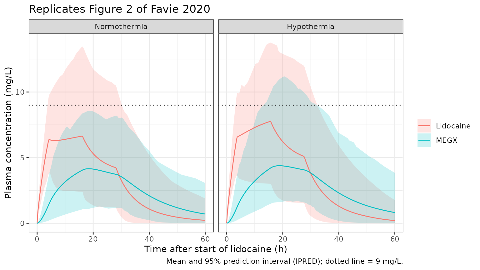
Peak lidocaine concentrations (Results 3.3)
peaks <- sim |>
  dplyr::group_by(arm, id) |>
  dplyr::summarise(peak = max(Cc), megx_end = Cc_megx[time == 60], .groups = "drop")

peak_tab <- peaks |>
  dplyr::group_by(arm) |>
  dplyr::summarise(
    median_peak = stats::median(peak),
    pct_over_9 = 100 * mean(peak > 9),
    pct_over_11 = 100 * mean(peak > 11),
    .groups = "drop"
  ) |>
  dplyr::mutate(
    paper_pct_over_9 = ifelse(arm == "Normothermia", 20.0, 31.8),
    paper_pct_over_11 = ifelse(arm == "Normothermia", 4.7, 12.8)
  )

peak_tab |>
  dplyr::rename(
    "Arm" = arm,
    "Median peak (mg/L)" = median_peak,
    "Simulated % > 9 mg/L" = pct_over_9,
    "Paper % > 9 mg/L" = paper_pct_over_9,
    "Simulated % > 11 mg/L" = pct_over_11,
    "Paper % > 11 mg/L" = paper_pct_over_11
  ) |>
knitr::kable(digits = 1)| Arm | Median peak (mg/L) | Simulated % > 9 mg/L | Simulated % > 11 mg/L | Paper % > 9 mg/L | Paper % > 11 mg/L |
|---|---|---|---|---|---|
| Hypothermia | 7.8 | 31 | 15.0 | 31.8 | 12.8 |
| Normothermia | 6.7 | 15 | 8.5 | 20.0 | 4.7 |
# Results 3.3: 'Both with and without TH, mean lidocaine peak plasma
# concentration was well below 9 mg/L'. Asserted on the cohort centre, which is
# robust to which subjects land in the tail.
stopifnot(all(peak_tab$median_peak < 9))
# TH reduces clearance, so exceedance is higher under TH in the paper; with 200
# per arm the binomial SE of each percentage is ~3 points and the paper's
# difference is ~12 points, so only the ordering is asserted.
stopifnot(
  peak_tab$pct_over_9[peak_tab$arm == "Hypothermia"] >
    peak_tab$pct_over_9[peak_tab$arm == "Normothermia"]
)
Salt-form reading of Table 1
The model is linear, so every individual concentration scales exactly
with the dose. Rescaling the simulated peaks by
1 / salt_base gives the same cohort dosed as if the Table 1
numbers were mg lidocaine base.
salt_tab <- dplyr::bind_rows(
  peaks |> dplyr::mutate(reading = "Hydrochloride (anhydrous), simulated above"),
  peaks |> dplyr::mutate(reading = "Base", peak = peak / salt_base)
) |>
  dplyr::group_by(reading, arm) |>
  dplyr::summarise(
    pct_over_9 = 100 * mean(peak > 9),
    pct_over_11 = 100 * mean(peak > 11),
    .groups = "drop"
  ) |>
  dplyr::mutate(
    paper_pct_over_9 = ifelse(arm == "Normothermia", 20.0, 31.8),
    paper_pct_over_11 = ifelse(arm == "Normothermia", 4.7, 12.8),
    abs_diff = abs(pct_over_9 - paper_pct_over_9) + abs(pct_over_11 - paper_pct_over_11)
  )

salt_tab |>
  dplyr::rename(
    "Dose reading" = reading,
    "Arm" = arm,
    "Simulated % > 9" = pct_over_9,
    "Paper % > 9" = paper_pct_over_9,
    "Simulated % > 11" = pct_over_11,
    "Paper % > 11" = paper_pct_over_11,
    "Sum of absolute differences" = abs_diff
  ) |>
knitr::kable(digits = 1)| Dose reading | Arm | Simulated % > 9 | Simulated % > 11 | Paper % > 9 | Paper % > 11 | Sum of absolute differences |
|---|---|---|---|---|---|---|
| Base | Hypothermia | 50.0 | 24.5 | 31.8 | 12.8 | 29.9 |
| Base | Normothermia | 33.5 | 11.5 | 20.0 | 4.7 | 20.3 |
| Hydrochloride (anhydrous), simulated above | Hypothermia | 31.0 | 15.0 | 31.8 | 12.8 | 3.0 |
| Hydrochloride (anhydrous), simulated above | Normothermia | 15.0 | 8.5 | 20.0 | 4.7 | 8.8 |
# Summed over the four published percentages, the hydrochloride reading was
# ~12 points from the paper and the base reading ~50 points when this was
# written; each percentage has a binomial SE of ~3 points at 200 per arm, so the
# ordering holds with a wide margin on any cohort draw.
misfit <- salt_tab |>
  dplyr::group_by(reading) |>
  dplyr::summarise(total = sum(abs_diff), .groups = "drop")
stopifnot(
  misfit$total[misfit$reading == "Base"] >
    misfit$total[misfit$reading != "Base"] + 15
)
The remaining differences (the normothermia arm in particular) are within what the reconstructed cohort can explain: the paper’s simulation replicated the 159 study neonates, whose individual weights, gestational and postnatal ages are not published, so the tail percentages are compared descriptively only. The paper also reports that “no accumulation of MEGX occurred”; in the simulation MEGX peaks around the end of maintenance phase I (PKNCA median Tmax ~20 h, below) and then declines through maintenance phase II and the washout.
PKNCA validation
The paper reports no NCA parameters, so PKNCA is used to summarise the simulated regimen per arm over the 28 h infusion course (Cmax, Tmax, AUC0-28), for lidocaine and MEGX separately. Doses are summed per subject and placed at time zero for the dose object.
dose_nca <- doses |>
  dplyr::left_join(cohort |> dplyr::select(id, arm), by = "id") |>
  dplyr::group_by(id, arm) |>
  dplyr::summarise(amt = sum(amt), .groups = "drop") |>
  dplyr::mutate(time = 0)

conc_nca <- sim |>
  dplyr::filter(!is.na(Cc), time <= 28) |>
  dplyr::select(id, arm, time, Cc, Cc_megx)

intervals <- data.frame(
  start = 0,
  end = 28,
  cmax = TRUE,
  tmax = TRUE,
  auclast = TRUE
)

run_nca <- function(conc_col) {
  d <- conc_nca |> dplyr::rename(conc = dplyr::all_of(conc_col))
  res <- PKNCA::pk.nca(PKNCA::PKNCAdata(
    PKNCA::PKNCAconc(d, conc ~ time | arm + id),
    PKNCA::PKNCAdose(dose_nca, amt ~ time | arm + id),
    intervals = intervals
  ))
  summary(res)
}

nca_lido <- run_nca("Cc")
nca_megx <- run_nca("Cc_megx")
knitr::kable(nca_lido, caption = "Lidocaine, 0-28 h")| start | end | arm | N | auclast | cmax | tmax |
|---|---|---|---|---|---|---|
| 0 | 28 | Hypothermia | 200 | 163 [39.7] | 7.70 [33.1] | 15.5 [3.50, 15.8] |
| 0 | 28 | Normothermia | 200 | 141 [41.9] | 6.92 [31.5] | 4.25 [4.00, 16.2] |
knitr::kable(nca_megx, caption = "MEGX, 0-28 h")| start | end | arm | N | auclast | cmax | tmax |
|---|---|---|---|---|---|---|
| 0 | 28 | Hypothermia | 200 | 80.2 [52.7] | 4.22 [48.6] | 19.9 [6.25, 28.0] |
| 0 | 28 | Normothermia | 200 | 76.8 [54.0] | 3.98 [49.7] | 19.8 [5.00, 28.0] |
Assumptions and deviations
-
PMA units. The Table 4 equations use PMA in days
about 280 days. The model takes the canonical
PAGEin weeks (the neonatal convention used by other library models) and formsPAGE * 7 - 280internally; the coefficient is unchanged. The linear PMA form reaches zero clearance at 19.3 weeks PMA and should not be used below the studied 25 weeks. -
Body temperature is protocolised. Per Table 4
footnote d,
BODYTEMPis 33.5 degC during TH with 0.4 degC/h rewarming and 36.5 degC otherwise, not a measured temperature. The timing of TH relative to lidocaine start in the simulation (TH from birth to 72 h, lidocaine from 24 h) is assumed. - Molar-mass conversion. The paper ran the analysis in umol, so the MEGX formation flux is molar. With doses in mg lidocaine base and concentrations in mg/L, the model multiplies the flux by 206.29 / 234.34 (MEGX / lidocaine molar masses). These constants are not printed in the paper.
-
Residual error. Additive (fixed 0.1 mg/L = LLQ/2)
plus proportional error per analyte is encoded as nlmixr2’s
add() + prop(); the paper does not say whether the two components were combined on the variance scale or summed on the SD scale. - No IIV covariances are reported, so the four etas are independent.
- Table 1 units and salt form. The Table 1 phase doses are read as mg/kg/h (see Dosing regimen). The paper converted lidocaine hydrochloride doses to base for the analysis but does not state whether the Table 1 regimen doses are hydrochloride or base. The simulation treats them as anhydrous lidocaine hydrochloride (base fraction 0.865), the reading that reproduces the paper’s exceedance percentages; the base reading over-predicts all four of them (see “Salt-form reading of Table 1”). The monohydrate factor (0.811) was not tested separately; it would lower all concentrations by a further 6%.
- Virtual cohort. The individual covariates of the paper’s 1113-subject simulation dataset are not published. GA was drawn uniformly within the preterm (25-36 weeks) and term (36-42 weeks) ranges, birth weight from an approximate GA-specific median birth-weight curve with 12% log-normal spread (not from the paper), and postnatal age at lidocaine start set to 1 day. The cohort size is capped at 200 per arm.
- Figure 1 (observed concentrations against the earlier van den Broek 2013 model) is not replicated: it uses a different, previously published model and the observed data are not available.
- Effectiveness and cardiac safety (Table 5, Section 3.4) are descriptive clinical outcomes, not modelled endpoints, and are not part of this model.