Tedatioxetine and its CYP2D6 metabolite Lu AA37208 (Frederiksen 2021)
Source:vignettes/articles/Frederiksen_2021_tedatioxetine.Rmd
Frederiksen_2021_tedatioxetine.RmdModel and source
- Citation: Frederiksen T, Areberg J, Schmidt E, Stage TB, Brosen K. Cytochrome P450 2D6 genotype-phenotype characterization through population pharmacokinetic modeling of tedatioxetine. CPT Pharmacometrics Syst Pharmacol. 2021;10(9):983-993. doi:10.1002/psp4.12635. PMCID: PMC8452298.
- Description: Joint parent + metabolite population PK model for oral tedatioxetine (Lu AA24530) and its major CYP2D6-dependent metabolite Lu AA37208, pooled across six phase I and one phase II study in 578 healthy subjects and patients with major depressive disorder (Frederiksen 2021). Tedatioxetine is dosed into an absorption-site compartment that drains by two competing first-order routes: intact drug into a two-compartment tedatioxetine disposition model (ka), and pre-systemic first-pass metabolism into an amount-only precursor pool (the intermediate Lu AA37209; k_precursor_luaa37208_form). The precursor converts to Lu AA37208 (k_luaa37208_form), which also receives systemic formation from the full tedatioxetine clearance (CL_CYP2D6) and then follows its own two-compartment disposition. All of the parent’s systemic clearance is assumed CYP2D6-mediated formation of Lu AA37208. Covariates retained: food state on the pre-systemic formation rate constant, and age (linear, centred at 37 years) on the metabolite clearance. Residual error is proportional and shared between the two analytes. Fit in NONMEM 7.4 (SAEM + importance sampling). The paper’s purpose was to quantify in vivo CYP2D6 activity per genotype from the individual formation-clearance estimates; the CYP2D6 genotype itself is NOT a covariate in the population PK model.
- Article: https://doi.org/10.1002/psp4.12635 (open access, PMC8452298)
Every structural equation and every parameter value below comes from
the paper’s Table 2 and from the final NONMEM control stream distributed
as supplementary material (PSP4-10-983-s004.docx). The
control stream is the authoritative source for the model
structure; Table 2 supplies the point estimates.
Population
Frederiksen 2021 pooled six phase I studies (dense PK sampling in healthy subjects) and one phase II dose-finding study (sparse sampling, at most three samples over six weeks in patients with major depressive disorder), for a total of 578 subjects: 220 healthy subjects and 358 patients with MDD. Tedatioxetine was given orally at 2-60 mg. The dataset held 5373 quantifiable tedatioxetine and 5449 quantifiable Lu AA37208 plasma concentrations. Baseline demographics (Table 1): median age 37 years (IQR 28-50, range 18-80), median weight 72 kg (range 42-140), 46% female. The CYP2D6 phenotype distribution (UM/NM/IM/PM) was 11/291/200/32 with 44 subjects ungenotyped. CYP2D6 genotype was used only in the downstream activity-score analysis, not as a population-PK covariate.
The same information is available programmatically via
readModelDb("Frederiksen_2021_tedatioxetine")()$population.
Model structure
The model is a joint parent + metabolite cascade with a
branched absorption site (Figure 2 and the
supplementary control stream $DES). The tedatioxetine
dosing compartment (depot) drains by two competing
first-order routes:
-
kacarries intact tedatioxetine into a two-compartment tedatioxetine disposition model (central/peripheral1, volumes V3 / V4); -
k_precursor_luaa37208_form(the control stream’sKGMET) represents pre-systemic first-pass metabolism, delivering drug into an amount-only pool of the intermediate Lu AA37209 (precursor_luaa37208).
The precursor converts to the metabolite Lu AA37208
at k_luaa37208_form (the control stream’s
KAMET), entering a two-compartment Lu AA37208 disposition
model (central_luaa37208 /
peripheral1_luaa37208, volumes V5 / V6). The metabolite
central compartment is additionally fed
systemically by the full tedatioxetine clearance
cl (CL_CYP2D6): all of the parent’s systemic elimination is
assumed to be CYP2D6-mediated formation of Lu AA37208.
Two covariates are retained: food state on the pre-systemic formation rate constant, and age (linear, centred at 37 years) on the metabolite clearance.
A note on the two absorption-branch rate constants
Table 2 of the paper and its executable control stream swap
the labels of the two metabolite-pathway rate constants. Table
2 lists a food-affected ka,met (11.1 /h fasted, 0.0286 /h
fed) and a single kg,met (0.0972 /h). The control stream,
however, applies the food effect to its KGMET – the
depot-to-precursor branch – and leaves KAMET, the
precursor-to-central conversion, food-independent. Matching by the food
split (only one rate is food-split in each document) and by the
$THETA initial estimates fixes the correspondence: the
depot-branching pre-systemic rate is the food-affected 11.1 /
0.0286 /h, and the precursor-to-metabolite conversion
rate is the 0.0972 /h value. This model follows the executable
control stream, which is the fitted object. The names used here
(k_precursor_luaa37208_form for the depot branch,
k_luaa37208_form for the conversion) reflect the structural
role each rate plays in the $DES, not the printed Table 2
labels.
Source trace
Every ini() entry carries an in-file comment naming its
Table 2 row (and its control-stream $THETA index); they are
collected here for review.
| Equation / parameter | Value | Source location |
|---|---|---|
d/dt(depot) (branched) |
n/a | control stream $DES A(1) |
d/dt(precursor_luaa37208) |
n/a | control stream $DES A(2) |
d/dt(central) |
n/a | control stream $DES A(3) |
d/dt(peripheral1) |
n/a | control stream $DES A(4) |
d/dt(central_luaa37208) |
n/a | control stream $DES A(5) |
d/dt(peripheral1_luaa37208) |
n/a | control stream $DES A(6) |
lka (ka) |
0.195 1/h | Table 2 |
lk_precursor_luaa37208_form fasted (KGMET) |
11.1 1/h | Table 2 ‘ka,met fasted’ |
e_fed_k_precursor_luaa37208_form |
fed 0.0286 1/h | Table 2 ‘ka,met fed’ |
lk_luaa37208_form (KAMET) |
0.0972 1/h | Table 2 ‘kg,met’ |
ltlag (ALAG) |
0.652 h | Table 2 |
lcl (CL_CYP2D6) |
30.5 L/h | Table 2 |
lvc (V3) |
1380 L | Table 2 |
lq (Q) |
39.1 L/h | Table 2 |
lvp (V4) |
507 L | Table 2 |
tvcl_luaa37208 (CLmet, age 37) |
11.9 L/h | Table 2 |
e_age_cl_luaa37208 |
-0.0830 L/h/yr | Table 2 ‘Age on CLmet’ |
lvc_luaa37208 (V5) |
33.1 L | Table 2 |
lq_luaa37208 (Qmet) |
0.940 L/h | Table 2 |
lvp_luaa37208 (V6) |
12.2 L | Table 2 |
| IIV variances | see Table 2 | Table 2 ‘IIV (%RSE)’ column, omega^2 = (CV/100)^2 |
cov(CL,V3) / cov(CLmet,V5)
|
0.079 / 0.372 | Table 2 covariance rows |
| Residual (proportional, shared) | 23.6% | Table 2 ‘Residual error’ |
Units
The control stream applies no unit conversion: with dose in mg and
volumes in L, A/V gives mg/L, so both Cc and
Cc_luaa37208 are in mg/L. The metabolite is carried in
tedatioxetine-mass equivalents (there is no molecular-weight factor on
the parent-to-metabolite flux in the control stream), so
Cc_luaa37208 is a mass-equivalent concentration rather than
a Lu AA37208 molar concentration.
mod <- readModelDb("Frederiksen_2021_tedatioxetine")
ui <- rxode2::rxode2(mod)
#> ℹ parameter labels from comments will be replaced by 'label()'
stopifnot(identical(ui$meta$units$concentration, "mg/L"))
Virtual cohort
Original observed data are not public. A cohort of 200 virtual subjects is simulated in each of the fasted and fed states, with age drawn to match the Table 1 distribution (median 37, IQR 28-50, range 18-80), so the food effect on the parent and the age effect on the metabolite are both exercised.
# rxode2's RNG is partitioned per solver thread, so this cohort is not
# byte-identical across machines with different thread counts. Every assertion
# below is written to hold for any cohort the model can produce, or uses the
# deterministic typical-value profiles (zeroRe) instead.
set.seed(20210901)
rxode2::rxSetSeed(20210901)

n_per_arm <- 200L
dose_mg <- 50
# Sampling grid to 336 h (~10.7 parent half-lives, kel = 30.5/1380 = 0.022 /h)
# so AUCinf extrapolation stays small for the closed-form gates below.
sample_times <- sort(unique(c(
  0, 0.5, 1, 2, 3, 4, 6, 8, 12, 16, 24, 36, 48, 72, 96, 120, 168, 240, 336
)))

draw_age <- function(n) {
  a <- round(rnorm(n, mean = 39, sd = 16))
  pmin(pmax(a, 18), 80)
}

make_arm <- function(n, fed, label, id_offset = 0L) {
  ids <- id_offset + seq_len(n)
  ages <- draw_age(n)
  covs <- tibble(id = ids, FED = fed, AGE = ages)
  dosing <- tibble(id = ids, time = 0, amt = dose_mg, evid = 1L, cmt = "depot")
  # Two endpoints are declared, so observation rows must name the OBSERVABLE
  # (cmt = "Cc"); cmt = "central" fails for a multi-endpoint model. Both Cc and
  # Cc_luaa37208 are returned as columns at every output row, so one set of
  # rows serves both analytes.
  obs <- tidyr::expand_grid(id = ids, time = sample_times) |>
    mutate(amt = NA_real_, evid = 0L, cmt = "Cc")
  bind_rows(dosing, obs) |>
    left_join(covs, by = "id") |>
    mutate(arm = label) |>
    arrange(id, time, desc(evid))
}

events <- bind_rows(
  make_arm(n_per_arm, 0, "Fasted", id_offset = 0L),
  make_arm(n_per_arm, 1, "Fed", id_offset = n_per_arm)
)

# Disjoint IDs across arms: rxSolve keys subjects on id.
stopifnot(length(intersect(
  events$id[events$arm == "Fasted"], events$id[events$arm == "Fed"]
)) == 0)
Simulation
sim <- rxode2::rxSolve(mod, events = events, keep = c("arm", "FED", "AGE")) |>
  as.data.frame()
#> ℹ parameter labels from comments will be replaced by 'label()'
stopifnot(all(c("Cc", "Cc_luaa37208", "arm") %in% names(sim)))
A deterministic typical-value replication (zeroRe) is
used for the structural gates and the figures:
mod_typical <- rxode2::zeroRe(mod)
#> ℹ parameter labels from comments will be replaced by 'label()'

typ_events <- function(fed, age, id) {
  bind_rows(
    tibble(id = id, time = 0, amt = dose_mg, evid = 1L, cmt = "depot"),
    tibble(id = id, time = c(0, seq(0.1, 336, by = 0.1)), amt = NA_real_, evid = 0L, cmt = "Cc")
  ) |>
    mutate(FED = fed, AGE = age) |>
    arrange(time, desc(evid))
}

ev_typ <- bind_rows(
  typ_events(0, 37, 1L) |> mutate(arm = "Fasted, age 37"),
  typ_events(1, 37, 2L) |> mutate(arm = "Fed, age 37"),
  typ_events(0, 60, 3L) |> mutate(arm = "Fasted, age 60")
)

sim_typ <- rxode2::rxSolve(mod_typical, events = ev_typ, keep = c("arm", "FED", "AGE")) |>
  as.data.frame()
#> ℹ omega/sigma items treated as zero: 'etalka', 'etalk_precursor_luaa37208_form', 'etalk_luaa37208_form', 'etalvc', 'etalcl', 'etalvc_luaa37208', 'etalcl_luaa37208'
#> Warning: multi-subject simulation without without 'omega'
Replicate published figures
The paper’s Figure 2 is a structural schematic rather than a data figure; the following typical-value profiles reproduce the qualitative behaviour the text describes: a slow tedatioxetine absorption (median parent t_max ~5-6 h) and a metabolite t_max “similar or shorter” driven by pre-systemic formation, plus the food and age effects that were the two retained covariates.
sim_typ |>
  select(time, arm, Tedatioxetine = Cc, `Lu AA37208` = Cc_luaa37208) |>
  filter(arm %in% c("Fasted, age 37", "Fed, age 37"), time > 0, time <= 72) |>
  pivot_longer(c(Tedatioxetine, `Lu AA37208`), names_to = "analyte", values_to = "conc") |>
  mutate(analyte = factor(analyte, levels = c("Tedatioxetine", "Lu AA37208"))) |>
  ggplot(aes(time, conc, colour = arm)) +
  geom_line(linewidth = 0.8) +
  facet_wrap(~analyte, scales = "free_y") +
  scale_y_log10() +
  labs(
    x = "Time (h)", y = "Plasma concentration (mg/L)", colour = NULL,
    title = "Typical-value tedatioxetine and Lu AA37208 profiles, fasted vs fed",
    caption = paste(
      "Food reduces the pre-systemic formation rate, raising parent exposure",
      "and lowering pre-systemic metabolite formation."
    )
  )
#> Warning in scale_y_log10(): log-10 transformation introduced infinite values.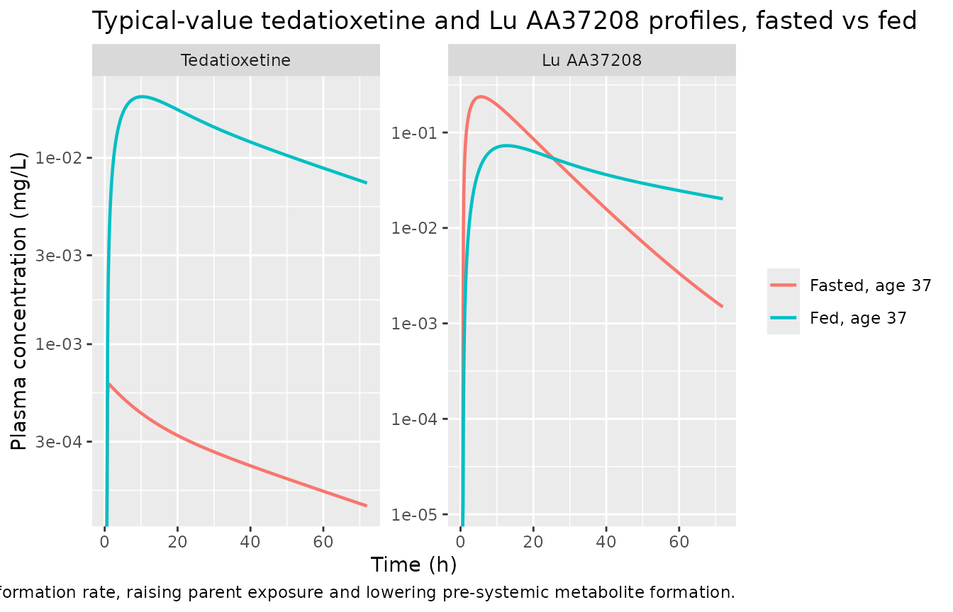
sim_typ |>
  filter(arm %in% c("Fasted, age 37", "Fasted, age 60"), time > 0, time <= 72) |>
  ggplot(aes(time, Cc_luaa37208, colour = arm)) +
  geom_line(linewidth = 0.8) +
  scale_y_log10() +
  labs(
    x = "Time (h)", y = "Lu AA37208 (mg/L)", colour = NULL,
    title = "Age effect on Lu AA37208 exposure (fasted)",
    caption = "Older subjects have lower metabolite clearance and higher metabolite exposure."
  )
#> Warning in scale_y_log10(): log-10 transformation introduced infinite values.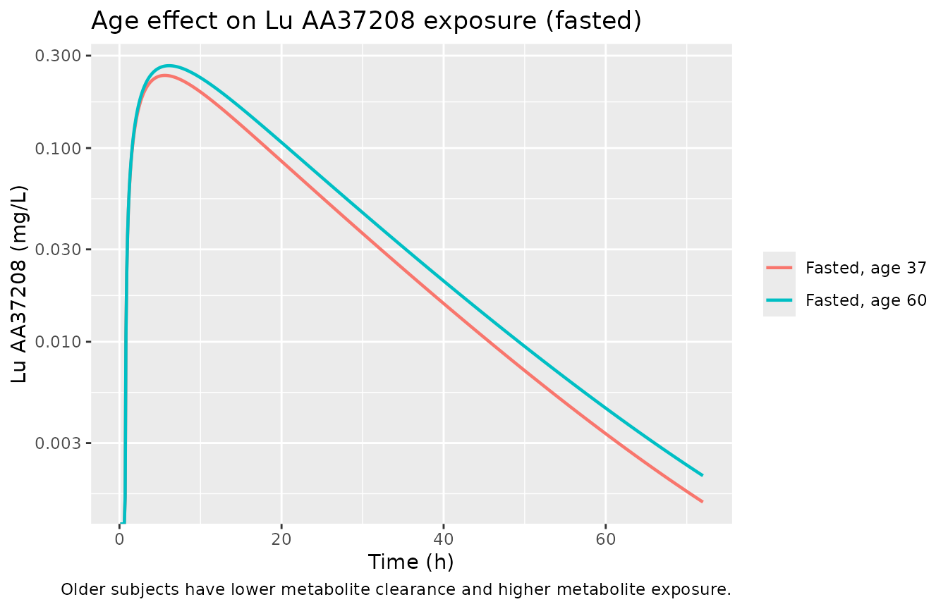
PKNCA validation
The paper reports no NCA summary table (Table 2 lists only model parameters), so the NCA here is validated against closed-form identities implied by the model structure rather than against a published table. One PKNCA block is run per analyte on the deterministic typical-value profiles.
make_nca <- function(conc_col) {
  d <- sim_typ |>
    filter(!is.na(.data[[conc_col]])) |>
    transmute(id, arm, time, Cc = .data[[conc_col]])
  # Anchor AUC at time zero (filter only on !is.na, never time > 0 / Cc > 0).
  d <- bind_rows(d, d |> distinct(id, arm) |> mutate(time = 0, Cc = 0)) |>
    distinct(id, arm, time, .keep_all = TRUE) |>
    arrange(id, arm, time)
  dose_df <- sim_typ |>
    distinct(id, arm) |>
    mutate(time = 0, amt = dose_mg)
  conc_obj <- PKNCA::PKNCAconc(d, Cc ~ time | arm + id)
  dose_obj <- PKNCA::PKNCAdose(dose_df, amt ~ time | arm + id)
  intervals <- data.frame(
    start = 0, end = Inf,
    cmax = TRUE, tmax = TRUE, auclast = TRUE, aucinf.obs = TRUE, half.life = TRUE
  )
  PKNCA::pk.nca(PKNCA::PKNCAdata(conc_obj, dose_obj, intervals = intervals))
}

nca_parent <- make_nca("Cc")
nca_met <- make_nca("Cc_luaa37208")

res_parent <- as.data.frame(nca_parent$result)
res_met <- as.data.frame(nca_met$result)

get_val <- function(res, arm_label, param) {
  res$PPORRES[res$arm == arm_label & res$PPTESTCD == param]
}
Closed-form gate 1: complete conversion to metabolite
In this model the parent’s only elimination pathway is
CYP2D6-mediated formation of Lu AA37208, and the pre-systemic branch
also forms Lu AA37208, so the entire absorbed dose is ultimately
recovered as metabolite (in tedatioxetine-mass equivalents).
Mass balance at infinite time therefore requires
cl_luaa37208 * AUCinf_met = dose, independent of food state
and of age (age changes cl_luaa37208 and
AUCinf_met in exactly compensating ways).
cl_met_age <- function(age) 11.9 + (age - 37) * (-0.0830)

mb <- tibble::tribble(
  ~arm,              ~age,
  "Fasted, age 37",  37,
  "Fed, age 37",     37,
  "Fasted, age 60",  60
) |>
  mutate(
    aucinf_met = vapply(arm, function(a) get_val(res_met, a, "aucinf.obs"), numeric(1)),
    cl_met = cl_met_age(age),
    product = cl_met * aucinf_met,
    pct_diff = 100 * (product - dose_mg) / dose_mg
  )

mb |>
  select(arm, cl_met, aucinf_met, product, pct_diff) |>
  rename(
    "Scenario" = arm, "CLmet (L/h)" = cl_met,
    "AUCinf metabolite (mg*h/L)" = aucinf_met,
    "CLmet x AUCinf" = product, "% diff from dose" = pct_diff
  ) |>
knitr::kable(digits = 3, caption = "Mass balance: all dose recovered as Lu AA37208.")| Scenario | CLmet (L/h) | AUCinf metabolite (mg*h/L) | CLmet x AUCinf | % diff from dose |
|---|---|---|---|---|
| Fasted, age 37 | 11.900 | 4.202 | 50.000 | 0.000 |
| Fed, age 37 | 11.900 | 4.202 | 49.998 | -0.003 |
| Fasted, age 60 | 9.991 | 5.004 | 50.000 | 0.000 |
Closed-form gate 2: parent clearance and food-dependent bioavailability
For the parent, cl * AUCinf_parent = dose * F_parent,
where the fraction of the oral dose reaching tedatioxetine central is
set by the branch competition at the depot,
F_parent = ka / (ka + k_precursor_luaa37208_form). Food
raises F_parent from ~1.7% (fasted, fast pre-systemic
branch) to ~87% (fed), which is the mechanism of the food effect.
ka <- 0.195
kgmet_fasted <- 11.1
kgmet_fed <- 0.0286
cl <- 30.5

fp <- tibble::tribble(
  ~arm,             ~kgmet,
  "Fasted, age 37", kgmet_fasted,
  "Fed, age 37",    kgmet_fed
) |>
  mutate(
    F_parent = ka / (ka + kgmet),
    aucinf_parent = vapply(arm, function(a) get_val(res_parent, a, "aucinf.obs"), numeric(1)),
    implied_cl = dose_mg * F_parent / aucinf_parent,
    pct_diff = 100 * (implied_cl - cl) / cl
  )

fp |>
  select(arm, F_parent, aucinf_parent, implied_cl, pct_diff) |>
  rename(
    "Scenario" = arm, "F_parent" = F_parent,
    "AUCinf parent (mg*h/L)" = aucinf_parent,
    "dose*F/AUC (L/h)" = implied_cl, "% diff from CL" = pct_diff
  ) |>
knitr::kable(digits = 4, caption = "Parent: dose*F/AUCinf recovers CL_CYP2D6 = 30.5 L/h.")| Scenario | F_parent | AUCinf parent (mg*h/L) | dose*F/AUC (L/h) | % diff from CL |
|---|---|---|---|---|
| Fasted, age 37 | 0.0173 | 0.0283 | 30.4977 | -0.0074 |
| Fed, age 37 | 0.8721 | 1.4294 | 30.5061 | 0.0199 |
Structural gate: metabolite t_max and the food effect
tmax_met_fasted <- get_val(res_met, "Fasted, age 37", "tmax")
cmax_parent_fasted <- get_val(res_parent, "Fasted, age 37", "cmax")
cmax_parent_fed <- get_val(res_parent, "Fed, age 37", "cmax")

tibble::tibble(
  Quantity = c(
    "Metabolite t_max, fasted (h)",
    "Parent Cmax fed / fasted"
  ),
  Value = c(tmax_met_fasted, cmax_parent_fed / cmax_parent_fasted)
) |>
knitr::kable(digits = 2, caption = "Structural behaviours described in the paper.")| Quantity | Value |
|---|---|
| Metabolite t_max, fasted (h) | 5.60 |
| Parent Cmax fed / fasted | 34.87 |
stopifnot(
  # Paper: metabolite t_max ~5-6 h (Introduction; presystemic formation).
  tmax_met_fasted >= 3 && tmax_met_fasted <= 8,
  # Food raises parent exposure substantially (reduced presystemic metabolism).
  cmax_parent_fed > cmax_parent_fasted
)
Stochastic cohort summary
The 200-per-arm cohort exercises the IIV and covariate distributions. Only distributional summaries are shown; per-subject extremes are not asserted on, because the extreme of a random cohort is not reproducible across rxode2 builds.
sim |>
  filter(time > 0) |>
  select(id, time, arm, Tedatioxetine = Cc, `Lu AA37208` = Cc_luaa37208) |>
  pivot_longer(c(Tedatioxetine, `Lu AA37208`), names_to = "analyte", values_to = "conc") |>
  mutate(analyte = factor(analyte, levels = c("Tedatioxetine", "Lu AA37208"))) |>
  group_by(analyte, arm, time) |>
  summarise(
    Q05 = quantile(conc, 0.05), Q50 = quantile(conc, 0.50),
    Q95 = quantile(conc, 0.95), .groups = "drop"
  ) |>
  filter(time <= 72) |>
  ggplot(aes(time, Q50, colour = arm, fill = arm)) +
  geom_ribbon(aes(ymin = Q05, ymax = Q95), alpha = 0.2, colour = NA) +
  geom_line(linewidth = 0.8) +
  facet_wrap(~analyte, scales = "free_y") +
  scale_y_log10() +
  labs(
    x = "Time (h)", y = "Plasma concentration (mg/L)", colour = NULL, fill = NULL,
    title = "Simulated cohort: median with 5th-95th percentile band",
    caption = paste0(n_per_arm, " subjects per arm.")
  )
#> Warning in scale_y_log10(): log-10 transformation introduced infinite values.
#> log-10 transformation introduced infinite values.
#> log-10 transformation introduced infinite values.
#> log-10 transformation introduced infinite values.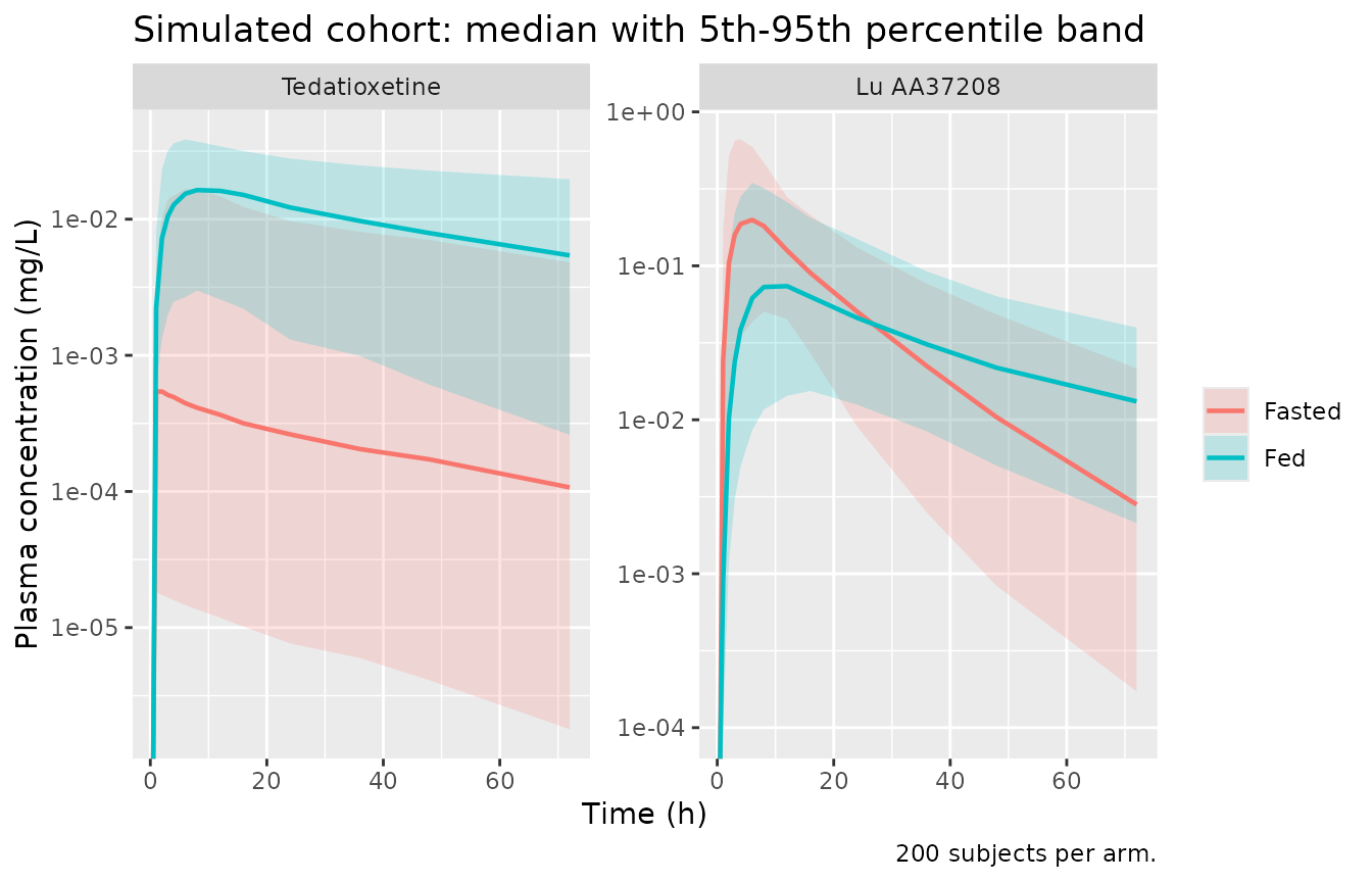
Assumptions and deviations
-
Between-subject variability scale. Table 2 reports
IIV as a percentage (“IIV (%RSE)”). The log-scale variance is encoded as
omega^2 = (CV/100)^2rather than the exact log-normalomega^2 = log((CV/100)^2 + 1). This reading is forced by the reported covariance: the CLmet-V5 covariance of 0.372, combined with the V5 (68.56%) and CLmet (55.05%) IIVs, gives a correlation of 0.986 under(CV/100)^2(valid) but a correlation greater than 1 (impossible) under the exact log-normal formula. The(CV/100)^2convention is therefore the only self-consistent reading of Table 2. -
The two absorption-branch rate constants are swapped between
Table 2 and the control stream. Table 2 labels the
food-affected rate (11.1 / 0.0286 /h)
ka,metand the single rate (0.0972 /h)kg,met, whereas the executable supplementary control stream applies the food effect to itsKGMET(the depot-to-precursor branch) and leavesKAMET(the precursor-to-central conversion) food-independent. The correspondence is fixed unambiguously by the food split and the$THETAinitial estimates. This model follows the executable control stream (the fitted object), so the food-affected rate is the depot-branching pre-systemic formation ratek_precursor_luaa37208_formand the 0.0972 /h rate is the precursor-to-metabolite conversion ratek_luaa37208_form. -
Residual error is log-additive in the source, encoded as
proportional. The control stream
$ERRORusesY = LOG(F + 0.001) + ERR(1), i.e. additive error on the log scale; Table 2 reports it as a proportional error of 23.6%. For the concentrations of interest the+0.001offset is negligible and the two forms coincide, so the canonical proportional form is used. A single sigma was estimated and applied to both analytes; nlmixr2 requires one residual parameter per endpoint, sopropSdandpropSd_luaa37208both carry the same 0.236 estimate. -
All parameters are apparent (per unknown
bioavailability). No intravenous data were available, so
clearances and volumes are apparent (
/F). The parent-to-metabolite split is modelled explicitly by the competing depot rate constants, and the extensive pre-systemic metabolism this implies (fastedF_parent~1.7%) is consistent with the paper’s characterization of tedatioxetine as a sensitive CYP2D6 substrate with pre-systemic metabolite formation. -
No molecular-weight conversion between analytes.
The control stream transfers a parent-mass amount directly into
central_luaa37208(CL/V3 * A(3)) with no MW factor, so the metabolite is carried in tedatioxetine-mass equivalents andCc_luaa37208is a mass-equivalent concentration. The equations are encoded exactly as in the control stream. -
The precursor pool holds Lu AA37209. The second
$MODEL COMP=(DEPOT)has no volume and no measured concentration (onlyS3=V3andS5=V5are set), so it isprecursor_luaa37208– the amount-onlyprecursor_<metab>construct – rather than acentral-style state with an invented volume. It holds the intermediate Lu AA37209 (Figure 1: tedatioxetine -> Lu AA37209 -> Lu AA37208). Theluaa37208metabolite suffix is registered ininst/references/compartment-names.md. - CYP2D6 genotype is not a population-PK covariate. The paper’s purpose was to estimate per-genotype CYP2D6 activity from the individual formation-clearance estimates of the fitted model, but the population PK model itself carries only food and age as covariates. The downstream activity-score regression is not part of this model file.
-
Age effect is additive on the linear clearance
scale. The control stream forms
CLMET = (THETA(9) + (AGE - 37) * THETA(14)) * exp(eta), an additive deviation on the linear clearance rather than the usual multiplicative power model. It is encoded exactly, centred at the median age of 37 years. -
Fixed-zero IIV. The control stream declares etas on
Q, V4, Qmet, V6 and the lag time but fixes their variance to 0
(
0 FIX); these parameters therefore carry no between-subject variability. -
Cohort composition. 200 virtual subjects per food
arm, age drawn to match the Table 1 distribution; the closed-form gates
use deterministic typical-value profiles (
zeroRe) and are asserted tightly, while the stochastic cohort is shown only as distributional summaries. ```