Tusamitamab ravtansine CYP downregulation IVIVE-PK (Pouzin 2023)
Source:vignettes/articles/Pouzin_2023_tusamitamab.Rmd
Pouzin_2023_tusamitamab.RmdModel and source
- Citation: Pouzin C, Teutonico D, Fagniez N, Ziti-Ljajic S, Perreard-Dumaine A, Pardon M, Klieber S, Nguyen L. Prediction of CYP Down Regulation after Tusamitamab Ravtansine Administration (a DM4-Conjugate), Based on an In Vitro-In Vivo Extrapolation Approach. Clin Pharmacol Ther. 2024;115(2):278-287. doi:10.1002/cpt.3102. PK layer: Pouzin C, Gibiansky L, Fagniez N, Chadjaa M, Tod M, Nguyen L. Integrated multiple analytes and semi-mechanistic population pharmacokinetic model of tusamitamab ravtansine, a DM4 anti-CEACAM5 antibody-drug conjugate. J Pharmacokinet Pharmacodyn. 2022;49(3):381-394. doi:10.1007/s10928-021-09799-0.
- Description: In vitro-in vivo extrapolation PK (IVIVE-PK) model of hepatic CYP3A4, CYP1A2 and CYP2B6 downregulation after tusamitamab ravtansine (SAR408701, anti-CEACAM5 IgG1-SPDB-DM4 ADC) in adults with advanced solid tumors (Pouzin 2023): indirect-turnover CYP abundance whose synthesis is reduced by unbound DM4 + Me-DM4 (inverse Hill, in vitro hepatocyte constants) and, for CYP3A4 only, mechanism-based inactivation by unbound DM4, driven by the integrated multi-analyte popPK model of Pouzin 2022 (DAR1-DAR8 ADC chains, naked antibody, DM4 and Me-DM4).
- Article: https://doi.org/10.1002/cpt.3102 (open access; published online 2023, issue dated February 2024)
- PK layer: https://doi.org/10.1007/s10928-021-09799-0, packaged on
its own as
Pouzin_2022_tusamitamab
Tusamitamab ravtansine (SAR408701) is an anti-CEACAM5 IgG1 antibody-drug conjugate carrying the maytansinoid DM4 through an SPDB linker. Free DM4 and its main metabolite methyl-DM4 (Me-DM4) circulate at low nanomolar concentrations. In human hepatocytes, Me-DM4 reduced CYP3A4, CYP1A2 and CYP2B6 mRNA in a concentration-dependent way, and in human liver microsomes DM4 was a mechanism-based (time-dependent) inactivator of CYP3A. Pouzin 2023 built an in vitro-in vivo extrapolation PK (IVIVE-PK) model to predict how far those in vitro effects reduce hepatic CYP abundance in patients.
The model has two layers:
PK layer. The integrated multi-analyte population PK model of Pouzin 2022 (DAR1-DAR8 ADC chains, naked antibody, DM4 and Me-DM4), which Pouzin 2023 used to generate the typical DM4 and Me-DM4 profiles. It is reproduced here unchanged from
Pouzin_2022_tusamitamab; see that model’s article for its own validation.-
IVIVE layer. An indirect turnover model for each CYP,
where the last (mechanism-based inactivation) term applies to CYP3A4 only. DM4 is assumed to downregulate with the same potency as Me-DM4, because DM4 was unstable in the hepatocyte incubation.
In the packaged model each CYP is carried as its abundance relative
to baseline (enzyme_3a4, enzyme_1a2,
enzyme_2b6, all starting at 1). Because the ODE is linear
in CYP, this is exactly the paper’s equation divided by
CYP0. The outputs pctchg_3a4,
pctchg_1a2 and pctchg_2b6 are the paper’s “CYP
abundance (% change)”, and abund_<cyp> are the
absolute abundances in pmol/mg microsomal protein.
Population
The IVIVE layer was not fitted to clinical data. Its constants are in vitro measurements: downregulation constants from fresh human hepatocytes of three donors (two evaluable for CYP1A2) treated for 72 h with Me-DM4 at 4-600 nM (Supplementary Table S1), mechanism-based inactivation constants from pooled human liver microsomes (50 donors), unbound fractions from binding studies (Table 1), and CYP turnover rates and baseline abundances from the Simcyp V22 library (Table 2). The DM4 and Me-DM4 drivers come from the Pouzin 2022 popPK model, which was fitted to 254 adults with advanced CEACAM5-expressing solid tumours in the first-in-human study TED13751 (NCT02187848).
The paper simulated two regimens with typical PK parameters: 100 mg/m^2 every 2 weeks (Q2W, up to 6 administrations) and 170 mg/m^2 every 3 weeks (Q3W, up to 4 administrations), each as a 1.5-hour intravenous infusion. It validated the approach externally in 8 evaluable patients who received SAR566658, an ADC with the same linker and payload, together with oral midazolam (Supplementary Material 3).
The same information is available programmatically via
readModelDb("Pouzin_2023_tusamitamab")()$population.
Source trace
Values for the PK layer are those of
Pouzin_2022_tusamitamab (Pouzin 2022 Table 4); its article
carries their source trace. The IVIVE layer:
| Equation / parameter | Value | Source location |
|---|---|---|
Indirect turnover dCYP/dt = kdeg*CYP0 - kdeg*CYP
|
- | Pouzin 2023 Methods, p. 280, and Figure 1 |
| Downregulation on synthesis (inverse Hill, DM4 + Me-DM4) | - | Pouzin 2023 Methods, p. 281, first displayed equation |
| Mechanism-based inactivation of CYP3A4 by DM4 | - | Pouzin 2023 Methods, p. 281, second displayed equation |
| CYP3A4 = downregulation + MBI combined | - | Pouzin 2023 Methods, ‘IVIVE-PK simulations’, p. 282 |
% change = 100 * (CYP - CYP0) / CYP0 |
- | Pouzin 2023 Methods, p. 282 |
kdeg_3a4 / kdeg_1a2 /
kdeg_2b6
|
0.0193 / 0.0183 / 0.0217 h^-1 (x 24 for 1/day) | Table 2 (Simcyp V22 library) |
cyp0_3a4 / cyp0_1a2 /
cyp0_2b6
|
137 / 52.0 / 21.6 pmol/mg protein | Table 2 (Simcyp V22 library) |
fu |
0.01 | Table 2 (in vitro binding assay) |
fuhep |
0.0909 | Table 2; Table 1 condition 3 |
fumic |
0.286 | Table 2; Table 1 condition 2 |
rmax_3a4 / rmax_1a2 /
rmax_2b6
|
0.0859 / 0.0194 / 0.212 | Table 2; Supplementary Table S1 donor means |
ec50_3a4 / ec50_1a2 /
ec50_2b6
|
0.0118 / 0.0159 / 0.0169 uM | Table 2; Supplementary Table S1 donor means |
kinact_3a4 |
6.12 h^-1 (x 24 for 1/day) | Table 2; Methods p. 280 |
ki_inact_3a4 |
2.3 uM | Table 2; Methods p. 280 |
Unbound fractions recomputed from Table 1
The two in vitro unbound fractions follow from the non-specific
binding study (fu,MIC1 = 0.500 at 0.100 mg/mL protein)
through the protein-scaling relation printed in the Methods. Recomputing
them confirms the Table 2 inputs:
fu_scale <- function(c_new, c_ref = 0.100, fu_ref = 0.500) {
  1 / (c_new / c_ref * (1 - fu_ref) / fu_ref + 1)
}
fu_recomputed <- c(fumic = fu_scale(0.250), fuhep = fu_scale(1.00))
fu_recomputed
#>      fumic      fuhep
#> 0.28571429 0.09090909
stopifnot(
  abs(fu_recomputed[["fumic"]] - 0.286) < 5e-4,
  abs(fu_recomputed[["fuhep"]] - 0.0909) < 5e-5
)
Virtual subject and dosing
The paper simulated typical profiles only, so the validation below
uses the typical subject (zeroRe()). Doses are entered in
umol of antibody (mg of ADC / 150, Pouzin 2022 Table 2) and split across
the eight DAR chains and the naked-antibody chain by the model’s
f() fractions, one dose row per chain. Pouzin 2023 does not
state the body-surface area behind its mg/m^2 doses; 1.79 m^2 is used,
the value with which Pouzin_2022_tusamitamab reproduces the
typical cycle-1 exposures of Pouzin 2022 Table 7.
bsa <- 1.79
chains <- c(paste0("dar", 1:8, "_central"), "central_nab")

make_events <- function(dose_mgm2, tau, n_doses, follow_up = 21, dt = 0.02) {
  amt <- dose_mgm2 * bsa / 150
  doses <- expand.grid(dose_index = seq_len(n_doses) - 1, cmt = chains, stringsAsFactors = FALSE) |>
    mutate(id = 1L, time = dose_index * tau, amt = amt, dur = 1.5 / 24, evid = 1L, dvid = NA_integer_) |>
    select(id, time, amt, dur, evid, cmt, dvid)
  obs <- data.frame(
    id = 1L, time = seq(0, (n_doses - 1) * tau + follow_up, by = dt),
    amt = NA_real_, dur = NA_real_, evid = 0L, cmt = NA_character_, dvid = 1L
  )
  bind_rows(doses, obs) |> arrange(time, desc(evid))
}

regimens <- list(
  "100 mg/m2 Q2W" = list(dose = 100, tau = 14, n = 6),
  "170 mg/m2 Q3W" = list(dose = 170, tau = 21, n = 4)
)

mod <- readModelDb("Pouzin_2023_tusamitamab")
mod_typ <- rxode2::zeroRe(rxode2::rxode2(mod))
#> ℹ parameter labels from comments will be replaced by 'label()'

solve_regimen <- function(ui, reg, label) {
  ev <- make_events(reg$dose, reg$tau, reg$n)
  rxode2::rxSolve(ui, ev, atol = 1e-10, rtol = 1e-10, returnType = "data.frame") |>
    mutate(regimen = label)
}

sim_typ <- bind_rows(lapply(names(regimens), function(nm) solve_regimen(mod_typ, regimens[[nm]], nm)))
#> ℹ omega/sigma items treated as zero: 'etalvc', 'etalvp', 'etalq', 'etalcladc', 'etalclnab', 'etalkdec1', 'etalcldm4', 'etalclmedm4', 'etalfrmedm4', 'etalfrdar1', 'etalfrdar2', 'etalfrdar3', 'etalfrdar4', 'etalfrdar5', 'etalfrdar6', 'etalfrdar7', 'etalfrnab'
#> ℹ omega/sigma items treated as zero: 'etalvc', 'etalvp', 'etalq', 'etalcladc', 'etalclnab', 'etalkdec1', 'etalcldm4', 'etalclmedm4', 'etalfrmedm4', 'etalfrdar1', 'etalfrdar2', 'etalfrdar3', 'etalfrdar4', 'etalfrdar5', 'etalfrdar6', 'etalfrdar7', 'etalfrnab'
Replicate Figure 2: CYP relative abundance
sim_typ |>
  select(time, regimen, CYP3A4 = pctchg_3a4, CYP1A2 = pctchg_1a2, CYP2B6 = pctchg_2b6) |>
  pivot_longer(starts_with("CYP"), names_to = "cyp", values_to = "pct") |>
  ggplot(aes(time, pct, colour = cyp)) +
  geom_line(linewidth = 0.8) +
  facet_wrap(~regimen, ncol = 1) +
  labs(x = "Time (days)", y = "CYP abundance (% change from baseline)", colour = NULL) +
  theme_bw()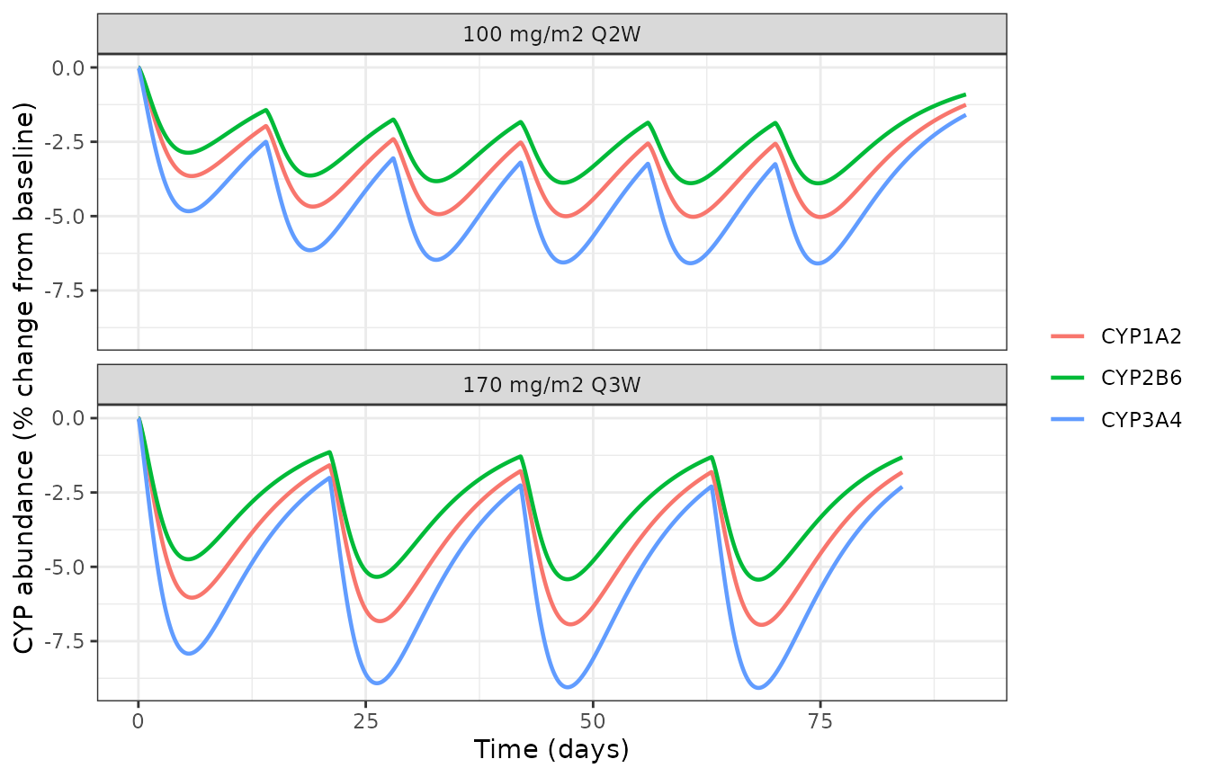
Replicates Figure 2 of Pouzin 2023: typical CYP3A4, CYP1A2 and CYP2B6 abundance (percent change from baseline) after 100 mg/m2 Q2W and 170 mg/m2 Q3W tusamitamab ravtansine.
Replicate Table 3: maximal CYP reduction
For each regimen the nadir is taken within the first dosing interval (cycle 1) and within the last simulated interval, which Pouzin 2023 calls steady state (reached at cycle 3 for Q2W and cycle 2 for Q3W). The time of the nadir is reported after the last dose, as in the paper.
nadir <- function(df, tau, n_doses, follow_up = 21) {
  windows <- list(
    "Cycle 1" = c(0, tau),
    "Steady state" = c((n_doses - 1) * tau, (n_doses - 1) * tau + follow_up)
  )
  bind_rows(lapply(names(windows), function(w) {
    lim <- windows[[w]]
    d <- df |> filter(time >= lim[1], time < lim[2])
    bind_rows(lapply(c(CYP3A4 = "pctchg_3a4", CYP1A2 = "pctchg_1a2", CYP2B6 = "pctchg_2b6"), function(col) {
      i <- which.min(d[[col]])
      data.frame(period = w, sim_pct = d[[col]][i], sim_day = d$time[i] - lim[1])
    }), .id = "cyp")
  }))
}

sim_tab3 <- bind_rows(lapply(names(regimens), function(nm) {
  nadir(filter(sim_typ, regimen == nm), regimens[[nm]]$tau, regimens[[nm]]$n) |>
    mutate(regimen = nm)
}))

# Pouzin 2023 Table 3
paper_tab3 <- tribble(
  ~regimen, ~period, ~cyp, ~paper_pct, ~paper_day,
  "100 mg/m2 Q2W", "Cycle 1", "CYP3A4", -4.7, 5.5,
  "100 mg/m2 Q2W", "Cycle 1", "CYP1A2", -3.6, 5.8,
  "100 mg/m2 Q2W", "Cycle 1", "CYP2B6", -2.8, 5.4,
  "100 mg/m2 Q2W", "Steady state", "CYP3A4", -6.4, 4.7,
  "100 mg/m2 Q2W", "Steady state", "CYP1A2", -4.9, 5.0,
  "100 mg/m2 Q2W", "Steady state", "CYP2B6", -3.8, 4.7,
  "170 mg/m2 Q3W", "Cycle 1", "CYP3A4", -7.7, 5.5,
  "170 mg/m2 Q3W", "Cycle 1", "CYP1A2", -5.9, 5.8,
  "170 mg/m2 Q3W", "Cycle 1", "CYP2B6", -4.6, 5.4,
  "170 mg/m2 Q3W", "Steady state", "CYP3A4", -8.8, 5.2,
  "170 mg/m2 Q3W", "Steady state", "CYP1A2", -6.8, 5.5,
  "170 mg/m2 Q3W", "Steady state", "CYP2B6", -5.3, 5.2
)

tab3 <- paper_tab3 |>
  left_join(sim_tab3, by = c("regimen", "period", "cyp")) |>
  mutate(pct_diff = 100 * (sim_pct / paper_pct - 1))

tab3 |>
  mutate(across(c(sim_pct, pct_diff), ~ round(.x, 2)), sim_day = round(sim_day, 1)) |>
  dplyr::rename(
    "Regimen" = regimen, "Period" = period, "CYP" = cyp,
    "Paper max reduction (%)" = paper_pct, "Simulated max reduction (%)" = sim_pct,
    "Paper nadir (days after dose)" = paper_day, "Simulated nadir (days after dose)" = sim_day,
    "Relative difference (%)" = pct_diff
  ) |>
knitr::kable()| Regimen | Period | CYP | Paper max reduction (%) | Paper nadir (days after dose) | Simulated max reduction (%) | Simulated nadir (days after dose) | Relative difference (%) |
|---|---|---|---|---|---|---|---|
| 100 mg/m2 Q2W | Cycle 1 | CYP3A4 | -4.7 | 5.5 | -4.83 | 5.5 | 2.85 |
| 100 mg/m2 Q2W | Cycle 1 | CYP1A2 | -3.6 | 5.8 | -3.65 | 5.9 | 1.46 |
| 100 mg/m2 Q2W | Cycle 1 | CYP2B6 | -2.8 | 5.4 | -2.87 | 5.5 | 2.43 |
| 100 mg/m2 Q2W | Steady state | CYP3A4 | -6.4 | 4.7 | -6.59 | 4.7 | 2.98 |
| 100 mg/m2 Q2W | Steady state | CYP1A2 | -4.9 | 5.0 | -5.03 | 5.0 | 2.62 |
| 100 mg/m2 Q2W | Steady state | CYP2B6 | -3.8 | 4.7 | -3.90 | 4.7 | 2.51 |
| 170 mg/m2 Q3W | Cycle 1 | CYP3A4 | -7.7 | 5.5 | -7.92 | 5.5 | 2.86 |
| 170 mg/m2 Q3W | Cycle 1 | CYP1A2 | -5.9 | 5.8 | -6.04 | 5.9 | 2.33 |
| 170 mg/m2 Q3W | Cycle 1 | CYP2B6 | -4.6 | 5.4 | -4.75 | 5.5 | 3.18 |
| 170 mg/m2 Q3W | Steady state | CYP3A4 | -8.8 | 5.2 | -9.07 | 5.2 | 3.09 |
| 170 mg/m2 Q3W | Steady state | CYP1A2 | -6.8 | 5.5 | -6.95 | 5.5 | 2.22 |
| 170 mg/m2 Q3W | Steady state | CYP2B6 | -5.3 | 5.2 | -5.43 | 5.2 | 2.48 |
# Typical-value solve of a deterministic system: every row is checked.
stopifnot(
  all(abs(tab3$pct_diff) < 6),
  all(abs(tab3$sim_day - tab3$paper_day) <= 0.2)
)
Every maximal reduction is reproduced to within 0.3 percentage points and every nadir time to within 0.1 day. The simulated reductions are consistently 1.5-3.2 % (relative) deeper than Table 3. The DM4 and Me-DM4 driver peaks match Pouzin 2022 to within 1 % (see the PKNCA check below), so the small offset is not explained by the dose or body-surface-area assumption; its source is not identified, and no parameter was adjusted.
Replicate Table 4 and Figure 3: contribution of each mechanism
Pouzin 2023 split the CYP3A4 reduction after 100 mg/m^2 Q2W into
three scenarios. Model 1 is the packaged model. Model 2 drops DM4 from
the downregulation driver; model 3 additionally drops the DM4
mechanism-based inactivation. Both are built from the packaged model by
replacing the corresponding model() lines.
ui_1 <- rxode2::rxode2(mod)
#> ℹ parameter labels from comments will be replaced by 'label()'
ui_2 <- rxode2::model(ui_1, cu_perp <- fu * Cc_medm4)
ui_3 <- rxode2::model(ui_2, kmbi_3a4 <- 0)
#> ! remove population parameter `kinact_3a4`
#> ! remove population parameter `ki_inact_3a4`
#> ! remove population parameter `fumic`

q2w <- regimens[["100 mg/m2 Q2W"]]
sim_scen <- bind_rows(
  "Model 1" = solve_regimen(rxode2::zeroRe(ui_1), q2w, "100 mg/m2 Q2W"),
  "Model 2" = solve_regimen(rxode2::zeroRe(ui_2), q2w, "100 mg/m2 Q2W"),
  "Model 3" = solve_regimen(rxode2::zeroRe(ui_3), q2w, "100 mg/m2 Q2W"),
  .id = "scenario"
)
#> ℹ omega/sigma items treated as zero: 'etalvc', 'etalvp', 'etalq', 'etalcladc', 'etalclnab', 'etalkdec1', 'etalcldm4', 'etalclmedm4', 'etalfrmedm4', 'etalfrdar1', 'etalfrdar2', 'etalfrdar3', 'etalfrdar4', 'etalfrdar5', 'etalfrdar6', 'etalfrdar7', 'etalfrnab'
#> ℹ omega/sigma items treated as zero: 'etalvc', 'etalvp', 'etalq', 'etalcladc', 'etalclnab', 'etalkdec1', 'etalcldm4', 'etalclmedm4', 'etalfrmedm4', 'etalfrdar1', 'etalfrdar2', 'etalfrdar3', 'etalfrdar4', 'etalfrdar5', 'etalfrdar6', 'etalfrdar7', 'etalfrnab'
#> ℹ omega/sigma items treated as zero: 'etalvc', 'etalvp', 'etalq', 'etalcladc', 'etalclnab', 'etalkdec1', 'etalcldm4', 'etalclmedm4', 'etalfrmedm4', 'etalfrdar1', 'etalfrdar2', 'etalfrdar3', 'etalfrdar4', 'etalfrdar5', 'etalfrdar6', 'etalfrdar7', 'etalfrnab'

sim_tab4 <- sim_scen |>
  group_by(scenario) |>
  group_modify(~ nadir(.x, q2w$tau, q2w$n)) |>
  ungroup() |>
  filter(cyp == "CYP3A4")

# Pouzin 2023 Table 4
paper_tab4 <- tribble(
  ~scenario, ~period, ~paper_pct, ~paper_day,
  "Model 1", "Cycle 1", -4.7, 5.5,
  "Model 2", "Cycle 1", -4.3, 5.8,
  "Model 3", "Cycle 1", -4.1, 6.1,
  "Model 1", "Steady state", -6.4, 4.7,
  "Model 2", "Steady state", -5.9, 5.0,
  "Model 3", "Steady state", -5.6, 5.2
)

tab4 <- paper_tab4 |>
  left_join(sim_tab4, by = c("scenario", "period")) |>
  mutate(pct_diff = 100 * (sim_pct / paper_pct - 1))

tab4 |>
  mutate(across(c(sim_pct, pct_diff), ~ round(.x, 2)), sim_day = round(sim_day, 1)) |>
  select(-cyp) |>
  dplyr::rename(
    "Scenario" = scenario, "Period" = period,
    "Paper max CYP3A4 reduction (%)" = paper_pct, "Simulated (%)" = sim_pct,
    "Paper nadir (days after dose)" = paper_day, "Simulated nadir (days after dose)" = sim_day,
    "Relative difference (%)" = pct_diff
  ) |>
knitr::kable()| Scenario | Period | Paper max CYP3A4 reduction (%) | Paper nadir (days after dose) | Simulated (%) | Simulated nadir (days after dose) | Relative difference (%) |
|---|---|---|---|---|---|---|
| Model 1 | Cycle 1 | -4.7 | 5.5 | -4.83 | 5.5 | 2.85 |
| Model 2 | Cycle 1 | -4.3 | 5.8 | -4.41 | 5.9 | 2.64 |
| Model 3 | Cycle 1 | -4.1 | 6.1 | -4.17 | 6.1 | 1.73 |
| Model 1 | Steady state | -6.4 | 4.7 | -6.59 | 4.7 | 2.98 |
| Model 2 | Steady state | -5.9 | 5.0 | -6.03 | 5.1 | 2.22 |
| Model 3 | Steady state | -5.6 | 5.2 | -5.70 | 5.3 | 1.79 |
ggplot(sim_scen, aes(time, pctchg_3a4, colour = scenario)) +
  geom_line(linewidth = 0.8) +
  labs(x = "Time (days)", y = "CYP3A4 abundance (% change from baseline)", colour = NULL) +
  theme_bw()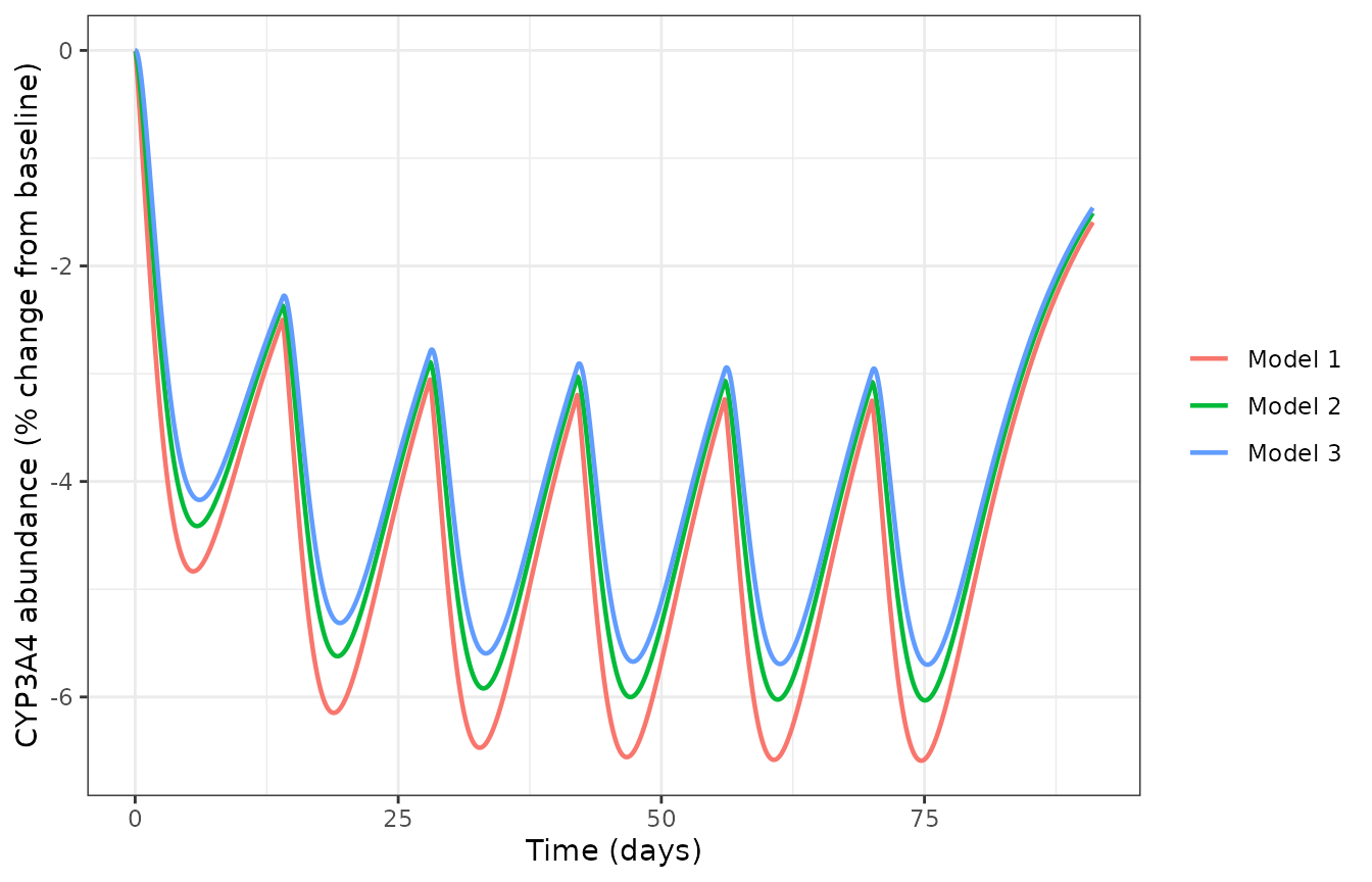
Replicates Figure 3 of Pouzin 2023: typical CYP3A4 abundance after 100 mg/m2 Q2W under model 1 (downregulation by Me-DM4 and DM4 plus DM4 MBI), model 2 (downregulation by Me-DM4 plus DM4 MBI) and model 3 (downregulation by Me-DM4 only).
Midazolam AUC ratio
Pouzin 2023 translated the maximal CYP3A4 reduction into a midazolam AUC ratio with a static PK-Sim PBPK simulation (15 mg oral midazolam). That PBPK model is not part of this package, but Supplementary Material 2 tabulates its output, which gives the ratio for the simulated nadirs by linear interpolation:
# Pouzin 2023 Supplementary Material 2
mdz <- data.frame(
  cyp3a4_change_pct = c(0, -5, -10, -15, -20, -25),
  auc_ratio = c(1.00, 1.07, 1.14, 1.23, 1.33, 1.44)
)
tab3 |>
  filter(cyp == "CYP3A4") |>
  mutate(midazolam_auc_ratio = approx(mdz$cyp3a4_change_pct, mdz$auc_ratio, xout = sim_pct)$y) |>
  transmute(
    "Regimen" = regimen, "Period" = period,
    "Simulated max CYP3A4 reduction (%)" = round(sim_pct, 2),
    "Interpolated midazolam AUC ratio" = round(midazolam_auc_ratio, 3)
  ) |>
knitr::kable()| Regimen | Period | Simulated max CYP3A4 reduction (%) | Interpolated midazolam AUC ratio |
|---|---|---|---|
| 100 mg/m2 Q2W | Cycle 1 | -4.83 | 1.068 |
| 100 mg/m2 Q2W | Steady state | -6.59 | 1.092 |
| 170 mg/m2 Q3W | Cycle 1 | -7.92 | 1.111 |
| 170 mg/m2 Q3W | Steady state | -9.07 | 1.127 |
All ratios stay below 1.25, the regulatory threshold for a weak CYP3A inhibitor, in line with the paper’s conclusion. The paper itself quotes 1.14, the ratio for a rounded worst case of a 10 % reduction.
PKNCA check of the DM4 and Me-DM4 drivers
The IVIVE layer is only as good as the DM4 and Me-DM4 profiles that drive it. Cycle-1 Cmax of both payload species after 100 mg/m^2 Q2W is compared with the typical values of Pouzin 2022 Table 7; Pouzin 2023 quotes the same DM4 Cmax (about 2.08 nM) in its Discussion.
q2w_c1 <- sim_typ |>
  filter(regimen == "100 mg/m2 Q2W", time <= 14) |>
  select(time, Cc_dm4, Cc_medm4) |>
  pivot_longer(c(Cc_dm4, Cc_medm4), names_to = "analyte", values_to = "conc") |>
  mutate(id = 1L, treatment = "100 mg/m2 Q2W") |>
  filter(!is.na(conc))

dose_c1 <- data.frame(
  id = 1L, time = 0, treatment = "100 mg/m2 Q2W",
  amt = 100 * bsa / 150
)
dose_c1 <- bind_rows(
  mutate(dose_c1, analyte = "Cc_dm4"),
  mutate(dose_c1, analyte = "Cc_medm4")
)

conc_obj <- PKNCA::PKNCAconc(q2w_c1, conc ~ time | treatment + analyte / id)
dose_obj <- PKNCA::PKNCAdose(dose_c1, amt ~ time | treatment + analyte + id)
intervals <- data.frame(start = 0, end = 14, cmax = TRUE, tmax = TRUE)
nca <- PKNCA::pk.nca(PKNCA::PKNCAdata(conc_obj, dose_obj, intervals = intervals))

sim_nca <- as.data.frame(nca$result) |>
  filter(PPTESTCD == "cmax") |>
  mutate(PPORRES = PPORRES * 1000) # uM -> nM

# Pouzin 2022 Table 7, cycle-1 Cmax (uM, shown here in nM)
ref_nca <- data.frame(
  treatment = "100 mg/m2 Q2W",
  analyte = c("Cc_dm4", "Cc_medm4"),
  cmax = c(0.00208, 0.00610) * 1000
)

cmp <- nlmixr2lib::ncaComparisonTable(
  sim_nca, ref_nca,
  by = c("treatment", "analyte"),
  params = "cmax",
  units = c(cmax = "nM")
)
knitr::kable(cmp)| NCA parameter | treatment | analyte | Reference | Simulated | % diff |
|---|---|---|---|---|---|
| Cmax (nM) | 100 mg/m2 Q2W | Cc_dm4 | 2.08 | 2.06 | -0.8% |
| Cmax (nM) | 100 mg/m2 Q2W | Cc_medm4 | 6.1 | 6.07 | -0.5% |
Between-subject spread (illustration)
Pouzin 2023 estimated no variability on the CYP layer and simulated typical profiles only. The PK layer does carry the Pouzin 2022 between-subject variability, so stochastic simulation shows how much the CYP3A4 nadir would spread from PK variability alone. This is an illustration, not a validation against the paper.
rxode2::rxSetSeed(20231114)
q3w <- regimens[["170 mg/m2 Q3W"]]
ev1 <- make_events(q3w$dose, q3w$tau, q3w$n, dt = 0.25)
ev_pop <- bind_rows(lapply(seq_len(100), function(i) mutate(ev1, id = i)))
sim_pop <- rxode2::rxSolve(rxode2::rxode2(mod), ev_pop, returnType = "data.frame")
#> ℹ parameter labels from comments will be replaced by 'label()'

band <- sim_pop |>
  group_by(time) |>
  summarise(
    p05 = quantile(pctchg_3a4, 0.05),
    p50 = quantile(pctchg_3a4, 0.50),
    p95 = quantile(pctchg_3a4, 0.95),
    .groups = "drop"
  )
typ_q3w <- filter(sim_typ, regimen == "170 mg/m2 Q3W")

ggplot(band, aes(time)) +
  geom_ribbon(aes(ymin = p05, ymax = p95), fill = "grey80") +
  geom_line(aes(y = p50), linetype = "dashed") +
  geom_line(data = typ_q3w, aes(y = pctchg_3a4), linewidth = 0.8) +
  labs(x = "Time (days)", y = "CYP3A4 abundance (% change from baseline)") +
  theme_bw()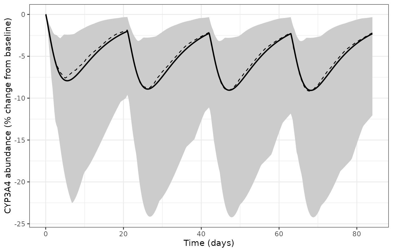
Typical-value (line) and 5th-95th percentile band (100 virtual patients, PK variability only) of CYP3A4 abundance after 170 mg/m2 Q3W.
Assumptions and deviations
-
PK layer carried from Pouzin 2022. Pouzin 2023
cites both Pouzin 2022 papers (the integrated model and its covariate
analysis) as the PK source but prints none of their parameters. The
typical integrated-model profile was used: its cycle-1 DM4 Cmax (2.08
nM, Pouzin 2022 Table 7) is the value Pouzin 2023 quotes in its
Discussion. The PK parameters, their between-subject variability and
residual errors are copied unchanged from
Pouzin_2022_tusamitamab, including that model’s compartment names. - No variability on the CYP layer. The paper estimated none (“only typical profiles were simulated”, Discussion), so none is added.
- Body-surface area. Not stated; 1.79 m^2 was used (see “Virtual subject and dosing”).
-
Infusion. The paper’s 1.5-hour infusion is applied
to every chain’s dose row with
dur. - Steady state. Taken as the last simulated dosing interval (the 6th Q2W or 4th Q3W dose), with a 21-day window after the last dose.
-
Time units.
kdegandkinactare printed per hour and are converted to per day (x 24) to match the PK layer. -
Relative-abundance states. The CYP states are
normalised to baseline (
enzyme_<cyp>(0) = 1), which is exact for this linear turnover model; absolute abundances are available asabund_<cyp>. - Midazolam. The PK-Sim midazolam PBPK model is not reproduced; its tabulated output (Supplementary Material 2) is interpolated instead.
- External validation not reproduced. The SAR566658 midazolam study used observed DM4 and Me-DM4 concentrations that are not published, so it cannot be re-run.
Errata
-
CYP3A4 equation. The mechanism-based inactivation
equation on p. 281 is printed with an unmodified synthesis term
kdeg * CYP3A4_0, but the Methods (“IVIVE-PK simulations”, p. 282) state that CYP3A4 reduction was simulated as the combination of downregulation and inactivation, and Table 4 (model 1 vs model 3) confirms both act together. The packaged CYP3A4 equation therefore combines the downregulated synthesis term with the inactivation term. -
Inactivation term form. The inactivation term is
printed as linear in concentration,
kinact * fu * C_DM4 / (KI * fu,MIC), rather than the saturablekinact * C / (KI + C)of the cited Yeo et al. form. It is implemented as printed; at the simulated unbound DM4 concentrations (about 2e-5 uM againstKI * fu,MIC= 0.66 uM) the two are indistinguishable. -
Me-DM4 in the inactivation term. The variable list
beneath the inactivation equation defines
C_MeDM4, but the equation and the text use DM4 only (Me-DM4 is a reversible CYP3A4 inhibitor, judged not relevant). Only DM4 is included. - CYP1A2 steady-state value. Table 3 and the Results give -6.8 % for CYP1A2 at steady state after 170 mg/m^2 Q3W; one sentence of the Discussion gives -6.6 %. Table 3 is used.
- Negative donor Rmax. Supplementary Table S1 lists a CYP1A2 Rmax of -0.00076 for donor 2; the mean 0.0194 used in Table 2 includes it.