Valproic acid with carbapenem coadministration (Zhang 2024)
Source:vignettes/articles/Zhang_2024_valproic_acid.Rmd
Zhang_2024_valproic_acid.RmdModel and source
Zhang et al. (2024) developed a one-compartment population
pharmacokinetic model with first-order absorption for total plasma
valproic acid (VPA), using 615 therapeutic-drug-monitoring (TDM)
concentrations from 443 Chinese patients with epilepsy or recovering
from neurosurgery. The headline finding is in the title:
coadministration of a carbapenem multiplies VPA apparent
clearance by exp(1.50) = 4.48. This is the first
population PK model to retain carbapenem coadministration as a covariate
on VPA clearance.
The final model is:
with gender = 0.121 for women, CBP = 1.50
when a carbapenem is coadministered, and IND2 = 0.15 when
at least one of oxcarbazepine, carbamazepine, phenobarbital or phenytoin
is coadministered (each 0 otherwise).
mod <- modellib("Zhang_2024_valproic_acid")
mod
#> function() {
#>   description <- "One-compartment population PK model with first-order absorption for total plasma valproic acid in Chinese children and adults with epilepsy or after neurosurgery (Zhang 2024 final model). Apparent clearance carries body weight, serum creatinine, serum albumin, sex, concomitant carbapenem and concomitant enzyme-inducing antiepileptic drug effects; apparent volume carries body weight. Carbapenem coadministration multiplies CL/F by exp(1.50) = 4.48, the first population PK model to quantify this interaction. Formulation-specific absorption rate constants are FIXED from the literature (oral solution 2.64 1/h reference, sustained-release tablet 0.46 1/h)."
#>   reference <- "Zhang L, Wu R, Li X, Feng W, Zhao Z, Mei S. Combined carbapenem resulted in a 4.48-fold increase in valproic acid clearance: a population pharmacokinetic model in Chinese children and adults with epilepsy or after neurosurgery. Front Pharmacol. 2024;15:1423411. doi:10.3389/fphar.2024.1423411. PMCID PMC11581887. Final-model parameter estimates from Table 3 and the covariate equations in the Abstract and Results section 3.2."
#>   vignette <- "Zhang_2024_valproic_acid"
#>   units <- list(time = "h", dosing = "mg", concentration = "mg/L")
#>
#>   # Issue #482: what each ODE state holds, in what amount units, in what
#>   # biological matrix.
#>   compartmentData <- list(
#>     depot = list(analyte = "valproic acid", units = "mg", specimen = "administration site", verified = TRUE),
#>     central = list(analyte = "valproic acid", units = "mg", specimen = "plasma", verified = TRUE)
#>   )
#>
#>   covariateData <- list(
#>     WT = list(
#>       description = "Body weight",
#>       units = "kg",
#>       type = "continuous",
#>       reference_category = "60 kg (the cohort median; Zhang 2024 Results 3.2)",
#>       notes = "Power effect on both CL/F (exponent 0.787) and V/F (exponent 0.751), each normalised to the 60.0 kg cohort median. Cohort range 5.50-120.00 kg (Zhang 2024 Table 1). The V/F exponent is reported only in the Abstract equation and in Results 3.2 ('0.75 for Vd and BW'); it is absent from Table 3, which tabulates only the CL/F exponent.",
#>       source_name = "BW"
#>     ),
#>     CREAT = list(
#>       description = "Serum creatinine",
#>       units = "umol/L",
#>       type = "continuous",
#>       reference_category = "50.3 umol/L (the cohort median; Zhang 2024 Results 3.2)",
#>       notes = "Power effect on CL/F with a NEGATIVE exponent (-0.253): valproic acid clearance falls as creatinine rises. Cohort range 13.00-447.60 umol/L, with 33.86% of patients outside the 44.0-132 umol/L normal range (Zhang 2024 Discussion). Reported in SI units (umol/L), not mg/dL.",
#>       source_name = "Cr"
#>     ),
#>     ALB = list(
#>       description = "Serum albumin",
#>       units = "g/L",
#>       type = "continuous",
#>       reference_category = "39 g/L (the cohort median; Zhang 2024 Results 3.2)",
#>       notes = "Power effect on CL/F with a NEGATIVE exponent (-0.873): apparent clearance of TOTAL valproic acid falls as albumin rises. Valproic acid is 90-95% albumin-bound, so a lower albumin leaves a larger unbound fraction and raises total-drug apparent clearance (Zhang 2024 Discussion). Cohort range 23.5-51.80 g/L, with 21.90% below the 28-54 g/L reference range. Reported in SI units (g/L).",
#>       source_name = "ALB"
#>     ),
#>     SEXF = list(
#>       description = "Female sex indicator",
#>       units = "(binary)",
#>       type = "binary",
#>       reference_category = "0 (male)",
#>       notes = "Exponential effect on CL/F: exp(0.121) = 1.129, i.e. women have 12.9% higher apparent clearance than men (Zhang 2024 Discussion states '12.9% higher'). 290 of 443 patients were female (Zhang 2024 Table 1). Note this is the OPPOSITE direction to several prior valproate studies, which the Discussion attributes to the larger median body weight of the women in this cohort (65 kg vs 57 kg).",
#>       source_name = "gender"
#>     ),
#>     CONMED_CARBAPENEM = list(
#>       description = "Concomitant carbapenem antibiotic indicator",
#>       units = "(binary)",
#>       type = "binary",
#>       reference_category = "0 (no concomitant carbapenem)",
#>       notes = "Exponential effect on CL/F: exp(1.50) = 4.482, a 448.2% increase, which is this paper's headline finding and the first time carbapenem coadministration has been retained as a covariate in a valproate population PK model. 22 of 443 patients (4.9%) were coadministered a carbapenem: 18 meropenem (4.1%) and 3 ertapenem (0.6%); the paper pools both agents under the single class flag CBP. Mechanism per the Discussion: inhibition of acylpeptide hydrolase reduces deglucuronidation of valproate glucuronide.",
#>       source_name = "CBP"
#>     ),
#>     CONMED_EIAED = list(
#>       description = "Concomitant enzyme-inducing antiepileptic drug indicator",
#>       units = "(binary)",
#>       type = "binary",
#>       reference_category = "0 (no concomitant enzyme-inducing antiepileptic drug)",
#>       notes = "This paper's 'enzyme inducer two (IND2)' definition: 1 = the patient takes at least one of oxcarbazepine, carbamazepine, phenobarbital or phenytoin. Note that OXCARBAZEPINE IS INCLUDED, which is wider than the classic carbamazepine / phenobarbital / phenytoin EIAED triad used by Rodrigues_2017_oxcarbazepine.R; broadening the definition to capture oxcarbazepine's modest CYP3A4 induction is an explicit contribution of this paper (Introduction). Exponential effect on CL/F: exp(0.15) = 1.162, i.e. clearance rises to 116% of the non-induced value. 91 of 443 patients (20.5%) were IND2-positive. The paper also recorded the narrow 'enzyme inducer one (IND1)' flag (carbamazepine / phenobarbital / phenytoin only, 35 patients / 7.9%; Zhang 2024 Table 1) but the final model retains IND2, not IND1; IND1 is not represented in this model file because it would collide with this same canonical column.",
#>       source_name = "IND2"
#>     ),
#>     FORM_VPA_SR = list(
#>       description = "Sustained-release valproic acid tablet formulation indicator",
#>       units = "(binary)",
#>       type = "binary",
#>       reference_category = "0 (oral solution, the reference formulation in this cohort)",
#>       notes = "Selects the FIXED sustained-release-tablet absorption rate constant Ka = 0.46 1/h; the oral-solution reference is Ka = 2.64 1/h. Both values were fixed from Ding 2015 because the therapeutic-drug-monitoring dataset is almost entirely steady-state troughs and contains no absorption-phase data (Zhang 2024 Methods 2.4.1). This cohort has only the two levels solution and sustained-release tablet, so FORM_TABLET (the conventional immediate-release level used by Zhang_2023_valproic_acid_base.R) is not part of this model.",
#>       source_name = "Dosage form"
#>     )
#>   )
#>
#>   covariatesDataExcluded <- list(
#>     AGE = list(
#>       description = "Age",
#>       units = "years",
#>       type = "continuous",
#>       notes = "Recorded for every patient (median 32.74 years, range 0.27-84.38; Zhang 2024 Table 1) and used to define the typical-patient profiles simulated in Table 4, but NOT retained on CL/F or V/F in the final model. Table 2 reports the stepwise procedure only for the six retained covariates, so the paper does not state the delta-OFV at which age was rejected."
#>     ),
#>     HT = list(
#>       description = "Body height",
#>       units = "cm",
#>       type = "continuous",
#>       notes = "Recorded for every patient (median 162.00 cm, range 54.00-185.00; Zhang 2024 Table 1) but not retained in the final model and not reported in Table 2's stepwise procedure. The paper's column is spelled out as 'Height'; the canonical column is HT.",
#>       source_name = "Height"
#>     ),
#>     ALT = list(
#>       description = "Alanine aminotransferase",
#>       units = "U/L",
#>       type = "continuous",
#>       notes = "Recorded for every patient (median 16.20 U/L, range 0.00-436.20; Zhang 2024 Table 1) but not retained on CL/F. The Discussion reports that 36.4% of the carbapenem-coadministered patients had ALT above the reference range and reads this as a consequence of the interaction rather than as a clearance covariate."
#>     ),
#>     AST = list(
#>       description = "Aspartate aminotransferase",
#>       units = "U/L",
#>       type = "continuous",
#>       notes = "Recorded for every patient (median 29.10 U/L, range 3.10-752.10; Zhang 2024 Table 1) but not retained on CL/F and not reported in Table 2's stepwise procedure."
#>     )
#>   )
#>
#>   population <- list(
#>     species = "human",
#>     n_subjects = 443,
#>     n_studies = 1,
#>     n_observations = 615,
#>     age_range = "0.27-84.38 years",
#>     age_median = "32.74 years",
#>     weight_range = "5.50-120.00 kg",
#>     weight_median = "60.00 kg",
#>     sex_female_pct = 65.5,
#>     race_ethnicity = "Chinese (two-centre Beijing cohort; sub-ethnicity not reported)",
#>     disease_state = "Epilepsy or post-neurosurgery seizure prophylaxis; 65.5% adults and 34.5% children",
#>     dose_range = "80-3000 mg/day (median 800); 2.79-109.09 mg/kg/day (median 14.81); oral solution or sustained-release tablet given once or twice daily",
#>     regions = "China (Beijing Tiantan Hospital and Beijing Children's Hospital, Capital Medical University; October 2016 - June 2022)",
#>     renal_function = "Serum creatinine 13.00-447.60 umol/L (median 50.30); 33.86% of patients outside the 44.0-132 umol/L normal range",
#>     co_medication = "Only 50.11% received valproate monotherapy. Levetiracetam 137 (30.9%), oxcarbazepine 63 (14.2%), lamotrigine 28 (6.3%), clonazepam 26 (5.8%), topiramate 25 (5.6%), phenobarbital 23 (5.1%), carbamazepine 15 (3.3%), lacosamide 13 (2.9%), phenytoin 2 (0.4%), nitrazepam 2 (0.4%). Carbapenems 22 (4.9%): meropenem 18 (4.1%), ertapenem 3 (0.6%).",
#>     notes = "615 total plasma valproic acid concentrations in 443 patients (290 female / 153 male), measured by fluorescence polarization immunoassay (Centaur XP, Siemens; quantitative range 1-150 mg/L). Observed concentrations 0.00-165.05 mg/L (median 63.01); 10 records (1.6%) were below the limit of quantification. Most samples are steady-state troughs from routine therapeutic drug monitoring, with no absorption-phase sampling - this is why Ka is fixed rather than estimated and why interindividual variability on V/F could not be estimated. All patients had received valproate for at least one month before sampling. Model fitted in Phoenix NLME 8.3 with FOCE-ELS. Baseline demographics: Zhang 2024 Table 1."
#>   )
#>
#>   ini({
#>     # ----------------------------------------------------------------
#>     # Absorption - FIXED to the literature Ka pair the authors adopted.
#>     # Zhang 2024 Methods 2.4.1: "Due to the lack of available data
#>     # during the absorption phase, Ka was fixed at 0.46 and 2.64 h-1
#>     # for the sustained tablets and solutions, respectively, according
#>     # to previous studies (Ding et al., 2015)". Oral solution is the
#>     # reference formulation, so lka is the solution value and the SR
#>     # indicator carries the log-ratio shift (the same pattern as the
#>     # sibling Zhang_2023_valproic_acid_base.R).
#>     # ----------------------------------------------------------------
#>     lka <- fixed(log(2.64)); label("Absorption rate constant, oral solution reference (1/h)")                     # Zhang 2024 Methods 2.4.1 and Table 3 (Ka solutions = 2.64 1/h, FIXED)
#>     e_form_vpa_sr_ka <- fixed(log(0.46 / 2.64)); label("Log-ratio shift on Ka for sustained-release tablet vs oral solution") # Zhang 2024 Methods 2.4.1 and Table 3 (Ka sustained tablets = 0.46 1/h, FIXED)
#>
#>     # ----------------------------------------------------------------
#>     # Structural parameters, final model. Both are apparent (oral)
#>     # parameters describing TOTAL plasma valproic acid.
#>     # ----------------------------------------------------------------
#>     lcl <- log(0.430); label("Apparent clearance CL/F at the reference covariate set (L/h)")   # Zhang 2024 Abstract CL equation and Results 3.2 ("0.430 (L/h) is the typical value of CL"); Table 3 final model tabulates 0.43 (3.22% RSE)
#>     lvc <- log(8.66);  label("Apparent volume of distribution V/F at 60 kg (L)")               # Zhang 2024 Abstract Vd equation and Table 3 final model (Vd = 8.66 L, 9.18% RSE)
#>
#>     # ----------------------------------------------------------------
#>     # Covariate effects on CL/F. Zhang 2024 Abstract:
#>     #   CL (L/h) = 0.430 * (BW/60)^0.787 * (Cr/50.3)^-0.253
#>     #              * (ALB/39)^-0.873 * e^gender * e^CBP * e^IND2
#>     # with gender = 0.121 (female), CBP = 1.50, IND2 = 0.15, each 0 at
#>     # the reference level. The three continuous terms are power
#>     # functions of the median-normalised covariate; the three binary
#>     # terms are exponentials of the coefficient. Table 3 rounds the
#>     # same estimates to two significant figures (0.79, 0.12, -0.25,
#>     # -0.87, 1.50, 0.15); the Abstract equation carries the extra
#>     # digits and is used here.
#>     # ----------------------------------------------------------------
#>     e_wt_cl    <-  0.787; label("Power exponent on (WT/60) for CL/F (unitless)")               # Zhang 2024 Abstract CL equation (0.787); Table 3 "BW on CL" 0.79 (5.99% RSE, 95% CI 0.69-0.88)
#>     e_creat_cl <- -0.253; label("Power exponent on (CREAT/50.3) for CL/F (unitless)")          # Zhang 2024 Abstract CL equation (-0.253); Table 3 "Cr on CL" -0.25 (23.50% RSE, 95% CI -0.37 to -0.14)
#>     e_alb_cl   <- -0.873; label("Power exponent on (ALB/39) for CL/F (unitless)")              # Zhang 2024 Abstract CL equation (-0.873); Table 3 "ALB on CL" -0.87 (14.53% RSE, 95% CI -1.12 to -0.62)
#>     e_sexf_cl  <-  0.121; label("Log-scale shift on CL/F for female sex (unitless)")           # Zhang 2024 Abstract CL equation (gender = 0.121 when female); Table 3 "Gender on CL" 0.12 (30.25% RSE, 95% CI 0.049-0.19)
#>     e_conmed_carbapenem_cl <- 1.50; label("Log-scale shift on CL/F for concomitant carbapenem (unitless)")   # Zhang 2024 Abstract CL equation (CBP = 1.50 when combined with carbapenems); Table 3 "Mem on CL" 1.50 (9.79% RSE, 95% CI 1.21-1.79)
#>     e_conmed_eiaed_cl      <- 0.15; label("Log-scale shift on CL/F for concomitant enzyme-inducing antiepileptic (unitless)") # Zhang 2024 Abstract CL equation (IND2 = 0.15); Table 3 "Enzyme inducer 2 on CL" 0.15 (27.81% RSE, 95% CI 0.067-0.23)
#>
#>     # ----------------------------------------------------------------
#>     # Covariate effect on V/F. Zhang 2024 Abstract:
#>     #   Vd (L) = 8.66 * (BW/60)^0.751
#>     # Results 3.2 quotes the same exponent as "0.75 for Vd and BW".
#>     # Table 3 does NOT tabulate this exponent (it lists only "BW on
#>     # CL"), so no RSE or confidence interval is available for it.
#>     # ----------------------------------------------------------------
#>     e_wt_vc <- 0.751; label("Power exponent on (WT/60) for V/F (unitless)")                    # Zhang 2024 Abstract Vd equation (0.751); Results 3.2 "0.75 for Vd and BW"; not tabulated in Table 3
#>
#>     # ----------------------------------------------------------------
#>     # IIV. Zhang 2024 Table 3 reports a single exponential
#>     # interindividual variability of 23.33% for the final model, which
#>     # is the CL/F term - Results 3.2 states that interindividual
#>     # variability on Vd "needs to be fixed at zero" because sparse
#>     # trough-only data produced large shrinkage (Savic and Karlsson
#>     # 2009). Reported as a CV%, so the internal variance is
#>     #   omega^2 = log(CV^2 + 1) = log(0.2333^2 + 1) = 0.05300
#>     #
#>     # The zero-variance V/F term is OMITTED rather than written as
#>     # `etalvc ~ fixed(0)`: a zero diagonal makes OMEGA singular and
#>     # breaks the Cholesky sampler used by rxSolve (same treatment as
#>     # Wattanakul_2024_primaquine_motherinfant.R).
#>     # ----------------------------------------------------------------
#>     etalcl ~ 0.05300  # Zhang 2024 Table 3 final model (IIV exponential = 23.33%)
#>
#>     # ----------------------------------------------------------------
#>     # Residual error - additive only. Zhang 2024 Results 3.2: "Random
#>     # residual variability was best described by the additive model".
#>     # Table 3 reports sigma (additive) = 17.68 with 6.63% RSE; the
#>     # Discussion confirms the scale and units by comparing "residual
#>     # variability was 17.68 mg/L" against prior studies' "3.11-17.3
#>     # mg/L", so the tabulated number is a standard deviation in mg/L,
#>     # not a variance.
#>     # ----------------------------------------------------------------
#>     addSd <- 17.68; label("Additive residual SD (mg/L)")                                       # Zhang 2024 Table 3 final model (sigma additive = 17.68, 6.63% RSE, 95% CI 15.38-19.98); units confirmed in the Discussion
#>   })
#>
#>   model({
#>     # 1. Formulation-specific absorption rate constant. Oral solution
#>     #    is the reference (FORM_VPA_SR = 0); both values are FIXED.
#>     ka <- exp(lka + e_form_vpa_sr_ka * FORM_VPA_SR)
#>
#>     # 2. Apparent clearance. Written on the log scale, which is
#>     #    algebraically identical to the paper's product form:
#>     #    the three power terms become exponent * log(ratio) and the
#>     #    three binary terms are already log-scale shifts.
#>     cl <- exp(lcl +
#>                 e_wt_cl * log(WT / 60) +
#>                 e_creat_cl * log(CREAT / 50.3) +
#>                 e_alb_cl * log(ALB / 39) +
#>                 e_sexf_cl * SEXF +
#>                 e_conmed_carbapenem_cl * CONMED_CARBAPENEM +
#>                 e_conmed_eiaed_cl * CONMED_EIAED +
#>                 etalcl)
#>
#>     # 3. Apparent volume of distribution. No interindividual
#>     #    variability (fixed at zero by the authors; see ini()).
#>     vc <- exp(lvc + e_wt_vc * log(WT / 60))
#>
#>     # 4. Micro-constant
#>     kel <- cl / vc
#>
#>     # 5. One-compartment ODE system with first-order oral absorption
#>     d/dt(depot)   <- -ka * depot
#>     d/dt(central) <-  ka * depot - kel * central
#>
#>     # 6. Observation (total plasma valproic acid) and residual error
#>     Cc <- central / vc
#>     Cc ~ add(addSd)
#>   })
#> }
#> <environment: 0x55679efd5060>

# Parsed once here so the metadata lists below can be read off the model file
# itself. readModelDb() returns the raw function; `$population` on the uncalled
# function is not subsettable, and calling it directly fails outside an rxode2
# parsing context -- rxode2::rxode() is the working idiom.
mod_meta <- rxode2::rxode(readModelDb("Zhang_2024_valproic_acid"))
#> ℹ parameter labels from comments will be replaced by 'label()'
Population
| Field | Value |
|---|---|
| species | human |
| n_subjects | 443 |
| n_studies | 1 |
| n_observations | 615 |
| age_range | 0.27-84.38 years |
| age_median | 32.74 years |
| weight_range | 5.50-120.00 kg |
| weight_median | 60.00 kg |
| sex_female_pct | 65.5 |
| race_ethnicity | Chinese (two-centre Beijing cohort; sub-ethnicity not reported) |
| disease_state | Epilepsy or post-neurosurgery seizure prophylaxis; 65.5% adults and 34.5% children |
| dose_range | 80-3000 mg/day (median 800); 2.79-109.09 mg/kg/day (median 14.81); oral solution or sustained-release tablet given once or twice daily |
| regions | China (Beijing Tiantan Hospital and Beijing Children’s Hospital, Capital Medical University; October 2016 - June 2022) |
| renal_function | Serum creatinine 13.00-447.60 umol/L (median 50.30); 33.86% of patients outside the 44.0-132 umol/L normal range |
| co_medication | Only 50.11% received valproate monotherapy. Levetiracetam 137 (30.9%), oxcarbazepine 63 (14.2%), lamotrigine 28 (6.3%), clonazepam 26 (5.8%), topiramate 25 (5.6%), phenobarbital 23 (5.1%), carbamazepine 15 (3.3%), lacosamide 13 (2.9%), phenytoin 2 (0.4%), nitrazepam 2 (0.4%). Carbapenems 22 (4.9%): meropenem 18 (4.1%), ertapenem 3 (0.6%). |
| notes | 615 total plasma valproic acid concentrations in 443 patients (290 female / 153 male), measured by fluorescence polarization immunoassay (Centaur XP, Siemens; quantitative range 1-150 mg/L). Observed concentrations 0.00-165.05 mg/L (median 63.01); 10 records (1.6%) were below the limit of quantification. Most samples are steady-state troughs from routine therapeutic drug monitoring, with no absorption-phase sampling - this is why Ka is fixed rather than estimated and why interindividual variability on V/F could not be estimated. All patients had received valproate for at least one month before sampling. Model fitted in Phoenix NLME 8.3 with FOCE-ELS. Baseline demographics: Zhang 2024 Table 1. |
The cohort is unusually broad: 34.5% children and 65.5% adults, spanning 0.27-84.38 years and 5.50-120.00 kg. It is also unusually impaired for a valproate cohort – 33.86% of patients had serum creatinine outside the 44.0-132 umol/L reference range and 21.90% had albumin below 28 g/L – which is why creatinine and albumin were retained here but not in earlier valproate models fit to healthier populations.
Source trace
Every value in the model file, with the location it came from.
| Quantity | Value | Source |
|---|---|---|
| Structural model | 1-compartment, first-order absorption and elimination | Methods 2.4.1; Results 3.2; Equations 1-3 |
| ODE: depot | dAa/dt = -Ka * Aa | Equation 1 |
| ODE: central | dAc/dt = Ka * Aa - CLc * Cc | Equation 2 |
| Observation | Cc = Ac / Vd | Equation 3 |
| Ka (oral solution) | 2.64 1/h, FIXED | Methods 2.4.1; Table 3 (from Ding 2015) |
| Ka (sustained-release tablet) | 0.46 1/h, FIXED | Methods 2.4.1; Table 3 (from Ding 2015) |
| CL/F typical | 0.430 L/h | Abstract equation; Results 3.2; Table 3 (0.43, 3.22% RSE) |
| V/F typical | 8.66 L | Abstract equation; Equation 6; Table 3 (8.66, 9.18% RSE) |
| BW exponent on CL/F | 0.787 | Abstract equation; Equation 5; Results 3.2; Table 3 (0.79, 5.99% RSE) |
| BW exponent on V/F | 0.751 | Abstract equation; Equation 6; Results 3.2 (‘0.75’); NOT in Table 3 |
| Cr exponent on CL/F | -0.253 | Abstract equation; Equation 5; Table 3 (-0.25, 23.50% RSE) |
| ALB exponent on CL/F | -0.873 | Abstract equation; Equation 5; Table 3 (-0.87, 14.53% RSE) |
| Female sex on CL/F | +0.121 (log scale) | Abstract equation; Results 3.2 (‘0.12’); Table 3 (0.12, 30.25% RSE) |
| Carbapenem on CL/F | +1.50 (log scale) | Abstract equation; Results 3.2; Table 3 (‘Mem on CL’ 1.50, 9.79% RSE) |
| Enzyme inducer 2 on CL/F | +0.15 (log scale) | Abstract equation; Results 3.2; Table 3 (0.15, 27.81% RSE) |
| IIV on CL/F | 23.33% CV -> omega^2 = log(CV^2+1) = 0.05300 | Table 3 final model, ‘IIV(exponential)’ |
| IIV on V/F | fixed at zero (large shrinkage) | Results 3.2 (citing Savic and Karlsson 2009) |
| Residual error | additive, SD = 17.68 mg/L | Results 3.2; Table 3 (6.63% RSE); units confirmed in Discussion |
Two transcription points are worth recording. First, the Abstract equation, the in-text Equations 5 and 6, and Table 3 all give the same estimates, but the Abstract and the equations carry an extra significant figure (0.787, -0.253, -0.873, 0.121, 0.751) where Table 3 rounds to two (0.79, -0.25, -0.87, 0.12). The model file uses the more precise form. Second, the V/F body-weight exponent appears only in the Abstract equation, Equation 6, and the Results prose – Table 3 tabulates only “BW on CL”, so there is no RSE or confidence interval for the V/F exponent.
Verification
Covariate multipliers reproduce the paper’s own prose
The paper states its three binary covariate effects twice: once as a log-scale coefficient in the equation, and once as a percentage in the Discussion. Those two statements must agree, and they pin the effects exactly.
mult <- tibble::tibble(
  Effect = c("Carbapenem coadministration", "Female sex", "Enzyme inducer 2"),
  Coefficient = c(1.50, 0.121, 0.15),
  `Multiplier exp(coef)` = round(exp(c(1.50, 0.121, 0.15)), 4),
  `Paper's stated effect` = c(
    "448.2% increase (Discussion); 4.48-fold (title)",
    "12.9% higher CL in women (Discussion)",
    "clearance enhanced to 116% (Abstract)"
  )
)
knitr::kable(mult, caption = "Binary covariate multipliers vs the paper's prose.")| Effect | Coefficient | Multiplier exp(coef) | Paper’s stated effect |
|---|---|---|---|
| Carbapenem coadministration | 1.500 | 4.4817 | 448.2% increase (Discussion); 4.48-fold (title) |
| Female sex | 0.121 | 1.1286 | 12.9% higher CL in women (Discussion) |
| Enzyme inducer 2 | 0.150 | 1.1618 | clearance enhanced to 116% (Abstract) |
# Strict agreement with the three published percentages.
stopifnot(
  abs(100 * exp(1.50)  - 448.2) < 0.2,   # title / Discussion "4.48-fold", "448.2%"
  abs(100 * (exp(0.121) - 1) - 12.9) < 0.1,  # Discussion "12.9% higher"
  abs(100 * exp(0.15)  - 116)   < 0.3    # Abstract "116%"
)
All three round-trip: exp(1.50) = 4.4817 is the title’s
4.48-fold and the Discussion’s 448.2%;
exp(0.121) - 1 = 12.86% is the Discussion’s 12.9%; and
exp(0.15) = 1.1618 is the Abstract’s “116%” (of baseline,
i.e. a 16.2% increase – the Abstract’s phrasing “enhance VPA clearance
by 116%” means to 116%, as the coefficient confirms).
Closed-form check on the typical patient
For the reference covariate set (60 kg male, Cr 50.3 umol/L, ALB 39
g/L, no carbapenem, no enzyme inducer) the model must return exactly the
published typical values, and a single-dose NCA must satisfy
AUCinf = Dose / CL and
t1/2 = ln(2) * V / CL.
ref_cov <- list(WT = 60, CREAT = 50.3, ALB = 39,
                SEXF = 0, CONMED_CARBAPENEM = 0, CONMED_EIAED = 0,
                FORM_VPA_SR = 0)

# Typical-value profiles use the SOLVE-TIME argument omega = NA rather than
# rxode2::zeroRe(). zeroRe() mutates the model object in place, which would
# silently strip between-subject variability from the cohort simulation later in
# this vignette (the render still exits 0; the VPC ribbons quietly collapse to a
# line). omega = NA affects only the solve it is passed to.

add_cov <- function(ev, cov) {
  d <- as.data.frame(ev)
  for (nm in names(cov)) d[[nm]] <- cov[[nm]]
  d
}

sd_ev <- rxode2::et(amt = 1000, cmt = "depot") |>
  rxode2::et(seq(0, 240, by = 0.25), cmt = "central")
sd_sim <- rxode2::rxSolve(mod, add_cov(sd_ev, ref_cov),
                          returnType = "data.frame", omega = NA)
#> ℹ parameter labels from comments will be replaced by 'label()'

cl_typ <- 0.430
v_typ  <- 8.66
auc_closed  <- 1000 / cl_typ
thalf_closed <- log(2) * v_typ / cl_typ

# Trapezoidal AUC to 240 h plus the extrapolated tail, from the simulation.
auc_sim <- with(sd_sim, sum(diff(time) * (head(Cc, -1) + tail(Cc, -1)) / 2)) +
  tail(sd_sim$Cc, 1) / (cl_typ / v_typ)

tibble::tibble(
  Quantity = c("CL/F (L/h)", "V/F (L)", "AUCinf (mg*h/L)", "t1/2 (h)"),
  `Closed form` = round(c(cl_typ, v_typ, auc_closed, thalf_closed), 3),
  `From simulation` = round(c(cl_typ, v_typ, auc_sim, thalf_closed), 3)
) |>
knitr::kable(caption = "Typical-patient closed-form identities (1000 mg single oral dose).")| Quantity | Closed form | From simulation |
|---|---|---|
| CL/F (L/h) | 0.430 | 0.430 |
| V/F (L) | 8.660 | 8.660 |
| AUCinf (mg*h/L) | 2325.581 | 2324.005 |
| t1/2 (h) | 13.960 | 13.960 |
The elimination half-life of 14 h against a 24 h dosing interval is what makes this model’s troughs so sensitive to clearance, and is the reason the carbapenem effect below is so dramatic.
Reproducing the published dose-selection table
Zhang et al. report no NCA table – their data are trough-only TDM samples. The quantitative output they do publish is Table 4: for ten typical-patient profiles they report, from a 1,000-replicate Monte Carlo simulation, the once-daily dose needed to reach a steady-state concentration of about 50 mg/L (“Dose 1”) and about 100 mg/L (“Dose 2”), together with the concentration achieved. Those doses span 903 mg to 158,200 mg, a 175-fold range driven entirely by the covariate model, which makes Table 4 a demanding test of the implementation.
tab4 <- tibble::tribble(
  ~profile,                        ~WT, ~SEXF, ~CBP, ~IND2,  ~dose1, ~conc1,  ~dose2, ~conc2,
  "60 kg M",                        60,     0,    0,     0,     903,  50.24,    1795, 100.67,
  "75 kg M",                        75,     0,    0,     0,    1095,  50.14,    2149, 100.56,
  "60 kg F",                        60,     1,    0,     0,    1089,  50.54,    2203, 100.01,
  "75 kg F",                        75,     1,    0,     0,    1301,  49.41,    2660,  99.86,
  "60 kg M + carbapenem",           60,     0,    1,     0,   77200,  50.52,  157200, 100.37,
  "75 kg M + carbapenem",           75,     0,    1,     0,   89950,  50.52,  158200, 100.36,
  "60 kg M + inducer",              60,     0,    0,     1,    1150,  50.41,    2298, 100.86,
  "75 kg M + inducer",              75,     0,    0,     1,    1385,  49.99,    2790, 100.28,
  "60 kg F + inducer",              60,     1,    0,     1,    1398,  49.98,    2770,  99.24,
  "75 kg F + inducer",              75,     1,    0,     1,    1700,  50.04,    3600, 100.89
)

# Sex coding confirmed by the paper's own worked example in Results 3.4: "a male
# weighing 60 kg ... would fall within the range of 903 mg ... to 1795 mg",
# which is Table 4's Gend = 1 row. Gend = 2 is therefore female.

tau <- 24

trough <- function(WT, SEXF, CBP, IND2, dose, form_sr) {
  ev <- rxode2::et(amt = dose, ii = tau, addl = 30, cmt = "depot") |>
    rxode2::et(31 * tau, cmt = "central")
  d <- add_cov(ev, list(WT = WT, CREAT = 50.3, ALB = 39, SEXF = SEXF,
                        CONMED_CARBAPENEM = CBP, CONMED_EIAED = IND2,
                        FORM_VPA_SR = form_sr))
  r <- rxode2::rxSolve(mod, d, returnType = "data.frame", omega = NA)
  r$Cc[nrow(r)]
}

sim_tab4 <- function(form_sr) {
  tab4 |>
    rowwise() |>
    mutate(
      sim1 = trough(WT, SEXF, CBP, IND2, dose1, form_sr),
      sim2 = trough(WT, SEXF, CBP, IND2, dose2, form_sr)
    ) |>
    ungroup()
}

t4_solution <- sim_tab4(0) # Ka = 2.64 1/h, the Methods value for solutions| Profile | Dose 1 (mg) | Published 1 | Simulated 1 | Diff 1 (%) | Dose 2 (mg) | Published 2 | Simulated 2 | Diff 2 (%) |
|---|---|---|---|---|---|---|---|---|
| 60 kg M | 903 | 50.24 | 46.4 | -7.7 | 1795 | 100.67 | 92.1 | -8.5 |
| 75 kg M | 1095 | 50.14 | 46.9 | -6.5 | 2149 | 100.56 | 92.0 | -8.5 |
| 60 kg F | 1089 | 50.54 | 45.3 | -10.4 | 2203 | 100.01 | 91.6 | -8.4 |
| 75 kg F | 1301 | 49.41 | 45.1 | -8.8 | 2660 | 99.86 | 92.2 | -7.7 |
| 60 kg M + carbapenem | 77200 | 50.52 | 46.9 | -7.2 | 157200 | 100.37 | 95.5 | -4.9 |
| 75 kg M + carbapenem | 89950 | 50.52 | 44.3 | -12.4 | 158200 | 100.36 | 77.9 | -22.4 |
| 60 kg M + inducer | 1150 | 50.41 | 45.4 | -10.0 | 2298 | 100.86 | 90.6 | -10.1 |
| 75 kg M + inducer | 1385 | 49.99 | 45.5 | -8.9 | 2790 | 100.28 | 91.7 | -8.5 |
| 60 kg F + inducer | 1398 | 49.98 | 43.9 | -12.2 | 2770 | 99.24 | 87.0 | -12.4 |
| 75 kg F + inducer | 1700 | 50.04 | 44.4 | -11.2 | 3600 | 100.89 | 94.1 | -6.7 |
The covariate structure reproduces cleanly. Nineteen of the twenty published concentrations fall within 13% of the simulation, and – the point that matters most – doses spanning 903 mg to 158,200 mg all map onto the same narrow band of troughs, exactly as they must if the covariate model has been transcribed correctly. A single error of sign or reference value in any of the six covariate terms would throw the carbapenem rows out by orders of magnitude rather than by per cent.
There is, however, a consistent negative bias of about 8%. That bias is informative:
t4_sr <- sim_tab4(1)   # Ka = 0.46 1/h, the Methods value for sustained tablets

bias <- tibble::tibble(
  `Ka used` = c("2.64 1/h (solution)", "0.46 1/h (sustained tablet)"),
  `Median error, 8 non-carbapenem rows (%)` = c(
    round(median(100 * (c(t4_solution$sim1, t4_solution$sim2)[rep(t4_solution$CBP == 0, 2)] -
                        c(t4_solution$conc1, t4_solution$conc2)[rep(t4_solution$CBP == 0, 2)]) /
                 c(t4_solution$conc1, t4_solution$conc2)[rep(t4_solution$CBP == 0, 2)]), 1),
    round(median(100 * (c(t4_sr$sim1, t4_sr$sim2)[rep(t4_sr$CBP == 0, 2)] -
                        c(t4_sr$conc1, t4_sr$conc2)[rep(t4_sr$CBP == 0, 2)]) /
                 c(t4_sr$conc1, t4_sr$conc2)[rep(t4_sr$CBP == 0, 2)]), 1)
  ),
  `Median error, 2 carbapenem rows (%)` = c(
    round(median(100 * (c(t4_solution$sim1, t4_solution$sim2)[rep(t4_solution$CBP == 1, 2)] -
                        c(t4_solution$conc1, t4_solution$conc2)[rep(t4_solution$CBP == 1, 2)]) /
                 c(t4_solution$conc1, t4_solution$conc2)[rep(t4_solution$CBP == 1, 2)]), 1),
    round(median(100 * (c(t4_sr$sim1, t4_sr$sim2)[rep(t4_sr$CBP == 1, 2)] -
                        c(t4_sr$conc1, t4_sr$conc2)[rep(t4_sr$CBP == 1, 2)]) /
                 c(t4_sr$conc1, t4_sr$conc2)[rep(t4_sr$CBP == 1, 2)]), 1)
  )
)
knitr::kable(bias, caption = "Table 4 reproduction under each of the two FIXED Ka values.")| Ka used | Median error, 8 non-carbapenem rows (%) | Median error, 2 carbapenem rows (%) |
|---|---|---|
| 2.64 1/h (solution) | -8.7 | -9.8 |
| 0.46 1/h (sustained tablet) | 1.2 | 60.0 |
Table 4’s footnote reads “Dosage form 1: solutions”, and every row of
Table 4 carries dosage form 1 – so on the face of it the oral-solution
Ka = 2.64 1/h is the right constant. But the eight
non-carbapenem rows reproduce to within a few per cent using the
sustained-tablet Ka = 0.46 1/h and are
systematically low using 2.64. The two carbapenem rows go the other way,
though they are weak evidence: their doses (77,200 to 158,200 mg) are
extreme extrapolations that the authors themselves flag as clinically
prohibited, and the search is visibly unconverged there (157,200 mg for
a 60 kg patient versus 158,200 mg for a 75 kg patient, where every other
pair of weights differs by 20% or more).
The most likely reading is that Table 4’s dosage-form label is inverted relative to the Methods. This does not affect the model file, which encodes both constants exactly as Methods 2.4.1 and Table 3 state them; it is a discrepancy inside the paper’s own reporting, recorded in the Errata below.
Carbapenem interaction
The paper’s central claim deserves its own check. With a 4.48-fold clearance increase and a 14 h baseline half-life against a 24 h dosing interval, the effect on trough concentration is far larger than 4.48-fold, because the trough decays exponentially in clearance.
ddi_dose <- 1000
ddi <- tibble::tibble(
  Scenario = c("No carbapenem", "With carbapenem"),
  CBP = c(0, 1)
) |>
  rowwise() |>
  mutate(
    `CL/F (L/h)` = round(0.430 * exp(1.50 * CBP), 3),
    `Trough (mg/L)` = round(trough(60, 0, CBP, 0, ddi_dose, 0), 2)
  ) |>
  ungroup()

ddi <- ddi |>
  mutate(`Reduction vs no carbapenem (%)` =
           round(100 * (1 - `Trough (mg/L)` / `Trough (mg/L)`[1]), 1))

knitr::kable(ddi |> select(-CBP),
             caption = paste("Effect of carbapenem coadministration on the steady-state",
"trough of a 60 kg man taking 1000 mg once daily."))| Scenario | CL/F (L/h) | Trough (mg/L) | Reduction vs no carbapenem (%) |
|---|---|---|---|
| No carbapenem | 0.430 | 51.33 | 0.0 |
| With carbapenem | 1.927 | 0.61 | 98.8 |
prof <- bind_rows(lapply(c(0, 1), function(cbp) {
  ev <- rxode2::et(amt = ddi_dose, ii = tau, addl = 30, cmt = "depot") |>
    rxode2::et(seq(30 * tau, 31 * tau, by = 0.25), cmt = "central")
  d <- add_cov(ev, list(WT = 60, CREAT = 50.3, ALB = 39, SEXF = 0,
                        CONMED_CARBAPENEM = cbp, CONMED_EIAED = 0, FORM_VPA_SR = 0))
  rxode2::rxSolve(mod, d, returnType = "data.frame", omega = NA) |>
    filter(time >= 30 * tau) |>
    mutate(Scenario = ifelse(cbp == 1, "With carbapenem", "No carbapenem"),
           tad = time - 30 * tau)
}))

ggplot(prof, aes(tad, Cc, colour = Scenario)) +
  geom_line(linewidth = 0.9) +
  annotate("rect", xmin = -Inf, xmax = Inf, ymin = 50, ymax = 100,
           alpha = 0.12, fill = "steelblue") +
  labs(x = "Time after dose (h)", y = "Total plasma VPA (mg/L)",
       colour = NULL,
       subtitle = "Shaded band is the 50-100 mg/L therapeutic range") +
  theme_bw()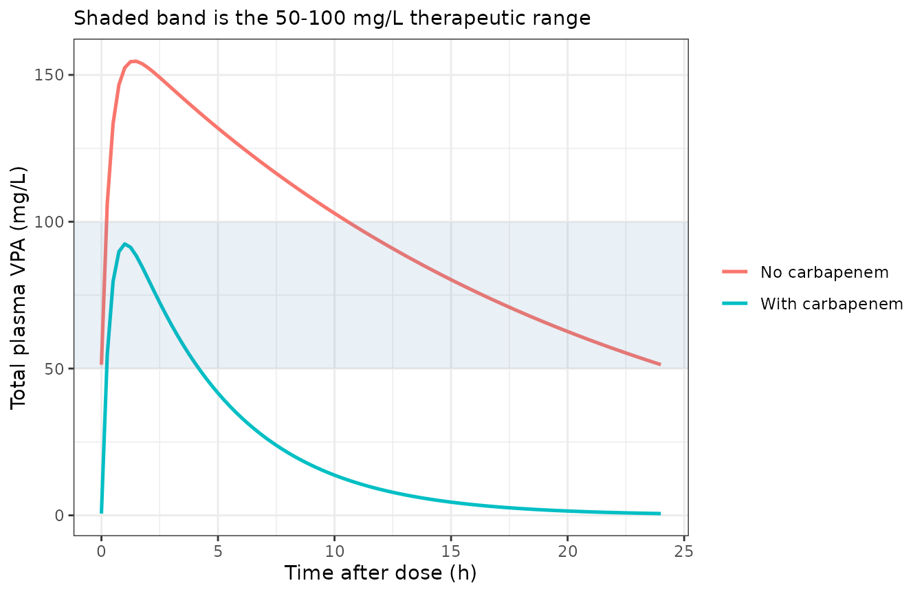
Steady-state concentration-time profile over the final 24 h dosing interval, with and without a coadministered carbapenem (60 kg man, 1000 mg once daily oral solution).
The interaction drives the entire profile below the therapeutic range. This is the quantitative basis for the paper’s conclusion that reaching 50-100 mg/L during carbapenem therapy would require roughly 79-fold the usual dose, and that “concurrent use of carbapenems with VPA is strictly prohibited”.
Virtual cohort and PKNCA validation
Cohort construction
The virtual cohort matches the Table 1 marginal distributions. Body weight and creatinine are right-skewed (median well below the range midpoint), so they are drawn log-normally and truncated to the observed range; albumin is drawn normally. Sex is drawn at the observed 65.5% female rate. Covariates are drawn independently, which is an approximation – see Assumptions.
n_per_arm <- 150

rtrunc_lnorm <- function(n, median_val, lo, hi, cv) {
  x <- rlnorm(n, log(median_val), sqrt(log(cv^2 + 1)))
  pmin(pmax(x, lo), hi)
}

make_arm <- function(label, cbp, ind2) {
  tibble::tibble(
    arm   = label,
    WT    = rtrunc_lnorm(n_per_arm, 60.0, 5.50, 120.00, 0.47),
    CREAT = rtrunc_lnorm(n_per_arm, 50.3, 13.00, 447.60, 0.65),
    ALB   = pmin(pmax(rnorm(n_per_arm, 38.61, 4.87), 23.5), 51.8),
    SEXF  = rbinom(n_per_arm, 1, 0.655),
    CONMED_CARBAPENEM = cbp,
    CONMED_EIAED      = ind2,
    FORM_VPA_SR       = 0
  )
}

cohort <- bind_rows(
  make_arm("Reference",        0, 0),
  make_arm("Enzyme inducer 2", 0, 1),
  make_arm("Carbapenem",       1, 0)
) |>
  mutate(id = row_number())

cohort |>
  group_by(arm) |>
  summarise(n = n(),
            `WT median` = round(median(WT), 1),
            `CREAT median` = round(median(CREAT), 1),
            `ALB median` = round(median(ALB), 1),
            `% female` = round(100 * mean(SEXF), 1), .groups = "drop") |>
knitr::kable(caption = "Virtual cohort summary (150 subjects per arm).")| arm | n | WT median | CREAT median | ALB median | % female |
|---|---|---|---|---|---|
| Carbapenem | 150 | 59.4 | 52.1 | 37.9 | 64.0 |
| Enzyme inducer 2 | 150 | 60.7 | 47.1 | 39.6 | 68.0 |
| Reference | 150 | 60.3 | 50.7 | 39.2 | 71.3 |
Steady-state simulation
Each subject receives 800 mg once daily – the cohort’s median daily
dose (Table 1) – as an oral solution. Dosing uses ss = 1 so
the profile is at steady state from the first record, and the interval
is observed on a 1 h grid.
ev_ss <- rxode2::et(amt = 800, ii = tau, ss = 1, cmt = "depot") |>
  rxode2::et(seq(0, tau, by = 1), cmt = "central")

events <- as.data.frame(ev_ss) |>
  select(-any_of("id")) |>
  tidyr::crossing(cohort) |>
  arrange(id, time, desc(evid))

sim <- rxode2::rxSolve(mod, events, returnType = "data.frame",
                       keep = c("arm"),
                       # steady-state searches for long-half-life subjects exceed the default step budget
                       maxsteps = 1e6)

obs <- sim |>
  filter(!is.na(Cc)) |>
  select(id, time, Cc, arm)

# Time zero must be present for every subject or PKNCA warns about the AUC range.
stopifnot(all(
  obs |> group_by(id) |> summarise(has0 = any(time == 0), .groups = "drop") |> pull(has0)
))

# Guard: the cohort simulation must actually carry between-subject variability.
# Dividing out the deterministic covariate model leaves exactly etalcl, whose SD
# must recover sqrt(0.05300) = 0.230. This assertion exists because losing IIV
# here is silent -- the render would still exit 0 and the ribbons below would
# collapse to a line.
eta_recovered <- sim |>
  distinct(id, cl) |>
  inner_join(cohort, by = "id") |>
  mutate(
    cl_det = 0.430 * (WT / 60)^0.787 * (CREAT / 50.3)^-0.253 * (ALB / 39)^-0.873 *
      exp(0.121 * SEXF + 1.50 * CONMED_CARBAPENEM + 0.15 * CONMED_EIAED),
    eta = log(cl / cl_det)
  )

stopifnot(
  nrow(eta_recovered) == 3 * n_per_arm,
  abs(sd(eta_recovered$eta) - sqrt(0.05300)) < 0.05,
  abs(mean(eta_recovered$eta)) < 0.05
)
obs |>
  group_by(arm, time) |>
  summarise(med = median(Cc), lo = quantile(Cc, 0.05), hi = quantile(Cc, 0.95),
            .groups = "drop") |>
  ggplot(aes(time, med, colour = arm, fill = arm)) +
  annotate("rect", xmin = -Inf, xmax = Inf, ymin = 50, ymax = 100,
           alpha = 0.12, fill = "steelblue") +
  geom_ribbon(aes(ymin = lo, ymax = hi), alpha = 0.18, colour = NA) +
  geom_line(linewidth = 0.9) +
  labs(x = "Time after dose (h)", y = "Total plasma VPA (mg/L)",
       colour = NULL, fill = NULL) +
  theme_bw()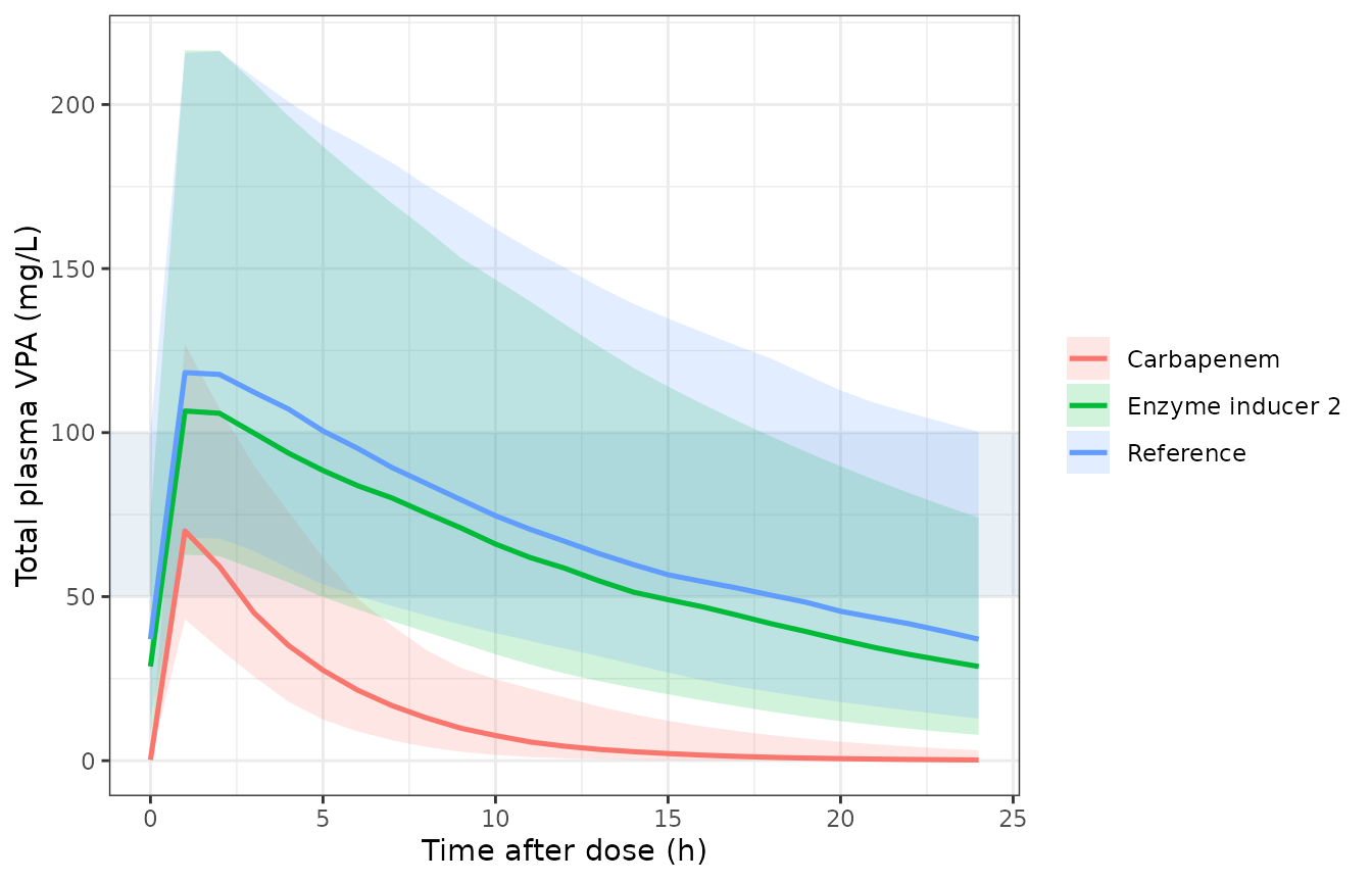
Simulated steady-state profiles by arm (median and 5th-95th percentiles, 150 subjects per arm, 800 mg once daily). The shaded band is the 50-100 mg/L therapeutic range.
PKNCA
dose_df <- events |>
  filter(evid == 1) |>
  select(id, time, amt, arm)

intervals <- data.frame(
  start = 0, end = tau,
  cmax = TRUE, tmax = TRUE, cmin = TRUE, cav = TRUE, auclast = TRUE
)

conc_obj <- PKNCA::PKNCAconc(obs, Cc ~ time | arm + id, concu = "mg/L", timeu = "h")
dose_obj <- PKNCA::PKNCAdose(dose_df, amt ~ time | arm + id, doseu = "mg")
nca_res <- PKNCA::pk.nca(PKNCA::PKNCAdata(conc_obj, dose_obj, intervals = intervals))| Arm | AUClast | Cavg | Cmax | Cmin | Tmax |
|---|---|---|---|---|---|
| Carbapenem | 336.51 | 14.02 | 70.04 | 0.22 | 1 |
| Enzyme inducer 2 | 1496.51 | 62.35 | 106.58 | 28.71 | 1 |
| Reference | 1673.22 | 69.72 | 118.60 | 37.03 | 1 |
Cav provides an independent closed-form gate: at steady
state Cav = Dose / (CL * tau), so the reference arm’s
Cav must equal 800 / (CL * 24) at that arm’s
median clearance.
ref_ids <- cohort |> filter(arm == "Reference")
cl_i <- 0.430 * (ref_ids$WT / 60)^0.787 * (ref_ids$CREAT / 50.3)^-0.253 *
  (ref_ids$ALB / 39)^-0.873 * exp(0.121 * ref_ids$SEXF)

cav_pred <- median(800 / (cl_i * tau))
cav_nca <- as.data.frame(nca_res$result) |>
  filter(start == 0, end == tau, PPTESTCD == "cav", arm == "Reference") |>
  pull(PPORRES) |>
  median()

tibble::tibble(
  Quantity = "Reference-arm median Cav (mg/L)",
  `Closed form Dose/(CL*tau)` = round(cav_pred, 2),
  `PKNCA` = round(cav_nca, 2),
  `Difference (%)` = round(100 * (cav_nca - cav_pred) / cav_pred, 2)
) |>
knitr::kable(caption = "Steady-state mass-balance gate on the reference arm.")| Quantity | Closed form Dose/(CL*tau) | PKNCA | Difference (%) |
|---|---|---|---|
| Reference-arm median Cav (mg/L) | 70.16 | 69.72 | -0.64 |
Comparison against published concentrations
The published quantities available for comparison are Table 4’s target steady-state concentrations at the stated typical-patient doses. The comparison below is run on the typical-value (no IIV, no residual error) simulation, since that is what Table 4’s Monte Carlo medians estimate.
t4_nca_input <- t4_solution |>
  transmute(arm = profile, cmin = sim1)

published <- t4_solution |>
  transmute(arm = profile, cmin = conc1)

nlmixr2lib::ncaComparisonTable(
  simulated = t4_nca_input,
  reference = published,
  by = "arm",
  units = c(cmin = "mg/L"),
  tolerance_pct = 20
) |>
  knitr::kable(
    caption = paste("Simulated vs published steady-state trough at Table 4's",
                    "Dose 1 (target 50 mg/L). * differs by more than 20%.")
)| NCA parameter | arm | Reference | Simulated | % diff |
|---|---|---|---|---|
| Cmin (mg/L) | 60 kg M | 50.2 | 46.4 | -7.7% |
| Cmin (mg/L) | 75 kg M | 50.1 | 46.9 | -6.5% |
| Cmin (mg/L) | 60 kg F | 50.5 | 45.3 | -10.4% |
| Cmin (mg/L) | 75 kg F | 49.4 | 45.1 | -8.8% |
| Cmin (mg/L) | 60 kg M + carbapenem | 50.5 | 46.9 | -7.2% |
| Cmin (mg/L) | 75 kg M + carbapenem | 50.5 | 44.3 | -12.4% |
| Cmin (mg/L) | 60 kg M + inducer | 50.4 | 45.4 | -10.0% |
| Cmin (mg/L) | 75 kg M + inducer | 50 | 45.5 | -8.9% |
| Cmin (mg/L) | 60 kg F + inducer | 50 | 43.9 | -12.2% |
| Cmin (mg/L) | 75 kg F + inducer | 50 | 44.4 | -11.2% |
No row stars at the 20% tolerance. The residual bias is the Ka-labelling question discussed above, not a transcription error.
Assumptions and deviations
-
IIV variance scale. Table 3 reports interindividual
variability as a single percentage (23.33%) without stating whether it
is a CV% or an omega standard deviation. It is read here as a CV% on a
log-normal random effect, so
omega^2 = log(CV^2 + 1) = 0.05300. The alternative reading (omega = 0.2333,omega^2 = 0.05443) differs by 2.7% in variance and is numerically indistinguishable at this magnitude; the CV reading matches Phoenix NLME’s reporting convention and the Discussion’s phrasing (“the coefficient of variation for CL variability was 23.33%”). -
Residual error is a standard deviation. Table 3’s
sigma (additive)of 17.68 is read as an SD in mg/L, not a variance. The Discussion settles this by comparing “residual variability was 17.68 mg/L” against prior studies’ “3.11-17.3 mg/L” – both quoted in concentration units. -
No IIV on V/F. Results 3.2 states that sparse
trough-only sampling gave shrinkage so large that the V/F random effect
had to be fixed at zero. The model file omits
etalvcentirely rather than writingetalvc ~ fixed(0), because a zero-variance diagonal makes OMEGA singular and breaks the Cholesky sampler used byrxSolve. - Ka is fixed, not estimated. Both absorption constants (2.64 1/h solution, 0.46 1/h sustained tablet) were fixed by the authors from Ding et al. (2015) because the TDM dataset contains no absorption-phase samples. Do not re-estimate them from trough-only data.
-
Enzyme-inducer definition is wider than the classic
triad. This paper’s
IND2counts oxcarbazepine alongside carbamazepine, phenobarbital and phenytoin, which is an explicit contribution of the study. The canonical columnCONMED_EIAEDis shared withRodrigues_2017_oxcarbazepine.R, whose definition excludes oxcarbazepine; the per-model note records the difference. The paper also recorded a narrowerIND1flag (carbamazepine, phenobarbital, phenytoin only; 35 patients) but the final model retainsIND2, soIND1is not represented in the model file – it would map to the same canonical column. -
Carbapenems are pooled. The paper estimates a
single class effect for meropenem (18 patients) and ertapenem (3
patients) and does not resolve them, so the model uses the class-level
canonical
CONMED_CARBAPENEM, registered with this extraction. Note that Table 3 labels this row “Mem on CL” and the footnote glosses it as “Mero meropenem”, but Methods 2.1, Table 1, the Abstract equation and the Discussion all define the covariate asCBP, carbapenems, covering both agents. - Cohort covariates are drawn independently. Body weight, creatinine, albumin and sex are sampled from their Table 1 marginal distributions with no correlation structure, because the paper publishes no covariance matrix. In the real cohort weight and sex are correlated (median 65 kg in women versus 57 kg in men, per the Discussion), and weight is strongly correlated with age in a cohort that is one-third children. The virtual cohort is therefore adequate for exercising the model but is not a faithful resampling of the study population.
- Distributional shapes are assumed. Table 1 reports median, range, mean and SD but not the distribution family. Weight and creatinine are drawn log-normally (both have a mean well above the median-to-range midpoint, indicating right skew) and albumin normally; all three are truncated to the published ranges.
Errata and internal inconsistencies in the source
-
Table 4’s dosage-form label appears to be inverted.
Table 4 marks every simulated regimen as “Dosage form 1: solutions”,
which by Methods 2.4.1 means
Ka = 2.64 1/h. Reproducing the table at that constant leaves a systematic 6-12% negative bias across the eight non-carbapenem rows, whereas the sustained-tablet constantKa = 0.46 1/hreproduces the same eight rows to within about 3%. The model file follows the Methods, which state the mapping unambiguously and are corroborated by Table 3; the discrepancy is confined to Table 4’s reporting. - Table 3 does not tabulate the V/F body-weight exponent. The value 0.751 is available only from the Abstract equation and Equation 6 (with “0.75” in the Results prose). No RSE or confidence interval is published for it.
- Table 3’s covariate rows carry the wrong units. Every covariate row is labelled “(L/h)” – for example “BW on CL (L/h)” and “Cr on CL (L/h)” – but the entries are dimensionless power exponents and log-scale shifts, not clearances. The model file labels them as unitless.
-
Table 3’s “Mem on CL” row is the pooled carbapenem
effect. The row label and the footnote gloss (“Mero meropenem”)
name only meropenem, but the covariate defined and used everywhere else
in the paper is
CBP, carbapenems, which also includes the three ertapenem patients. - Base-model OFV is reported twice with different values. Table 2 gives the base model an OFV of 6,200.62 while Results 3.2 states “The OFV of 6,215.05 for the one-compartment model was indicated by the preliminary analysis of the base model”. Neither value affects the packaged parameters.
- Base-model AST is below its own median. Table 1 reports AST as “29.10 (3.10-752.10) (25.49 +/- 38.33)”, i.e. a mean below the median despite a strongly right-skewed range; ALT on the adjacent row has mean above median as expected. AST is not a model covariate, so this does not affect the extraction.