Vonoprazan (Mulford 2026) • nlmixr2lib

Model and source

Citation: Mulford DJ, Facius A, Witt G, Howden CW, Wagner T, Leifke E, Scarpignato C. Development and Use of a Population Pharmacokinetic Model for Characterizing the Pharmacokinetics of Vonoprazan in Pediatric Patients. CPT Pharmacometrics Syst Pharmacol. 2026;15:e70291. doi:10.1002/psp4.70291. Structural detail and covariate centering values taken from the Supporting Information Model Code (the final-model NONMEM control stream, PSP4-15-e70291-s001.docx).
Article: https://doi.org/10.1002/psp4.70291
Supporting Information (Model Code, Tables S1-S4, Figures S1-S3): https://www.ebi.ac.uk/europepmc/webservices/rest/PMC13316124/supplementaryFiles

Mulford 2026 develops a population pharmacokinetic model for vonoprazan, a potassium-competitive acid blocker approved in adults but not, as of June 2026, for pediatric use. The model was built iteratively in a learn-and-confirm sequence: Model 1 from eight adult studies, Model 2 after adding the adolescent study VPED-102, and Model 3 after adding the child study VPED-103. The structure never changed across the three iterations – each posterior predictive check found no systematic deviation – so only the parameter estimates were updated. Table 1 of the paper prints all three parameter sets side by side, and Results 3.1 directs the reader to the rightmost column (Children) for the numerical estimates. That column, Model 3, is what Mulford_2026_vonoprazan packages.

This paper contributes two model files:

mod     <- readModelDb("Mulford_2026_vonoprazan")
mod_mat <- readModelDb("Mulford_2026_vonoprazan_maturation")

Mulford_2026_vonoprazan – Model 3 as fitted, the final model for the observed 6-to-54-year age range.
Mulford_2026_vonoprazan_maturation – Model 3 extended (Methods 2.4.2) with a sigmoid organ-maturation factor on clearance, used to project exposure in infants and children aged 1 month to under 6 years, where no vonoprazan data exist. The maturation constants are literature values, not estimates.

Population

The pooled analysis dataset (Table S1) holds 392 subjects and 8201 quantifiable plasma concentrations from ten studies across Japan, Europe, China and the United States:

Adults, n = 354, all healthy volunteers, eight phase 1 studies, doses 1 mg to 120 mg including a 20 mg twice-daily arm. Age mean 28.2 years (SD 7.46, range 18-54); weight mean 68.3 kg (SD 10.7, range 50.1-114), median 66 kg.
Adolescents, n = 17, patients with gastroesophageal reflux disease, study VPED-102 (NCT05343364), 10 mg (n = 9) or 20 mg (n = 8) once daily, oral tablet. Age mean 14.6 years (SD 1.69, range 12-17); weight mean 72.0 kg (SD 25.6, range 42.3-132), median 64 kg. One 15-year-old weighing 132 kg sits at the top of that distribution and is why the adolescent mean weight exceeds the adult mean.
Children, n = 21, patients with gastroesophageal reflux disease, study VPED-103 (NCT06106022), 10 mg (n = 10) or 20 mg (n = 11) once daily, oral tablet, sparse sampling. Age mean 8.76 years (SD 1.76, range 6.0-11); weight mean 36.2 kg (SD 12.4, range 20.7-71.2), median 32 kg.

About 5% of concentrations were below the limit of quantification and were retained through the Beal M3 method; Table S4 reports the sensitivity analysis without M3. The female fraction and the race distribution are not reported numerically. Race was screened graphically (Figure S3) and not retained.

The same information is available programmatically:

str(rxode2::rxode(mod)$population)
#> ℹ parameter labels from comments will be replaced by 'label()'
#> List of 11
#>  $ species       : chr "human"
#>  $ n_subjects    : int 392
#>  $ n_studies     : int 10
#>  $ n_observations: int 8201
#>  $ age_range     : chr "6-54 years"
#>  $ weight_range  : chr "20.7-132 kg"
#>  $ weight_median : chr "66 kg (adults), 64 kg (adolescents), 32 kg (children)"
#>  $ disease_state : chr "healthy volunteers (all eight adult studies) and patients with gastroesophageal reflux disease (the adolescent "| __truncated__
#>  $ dose_range    : chr "1-120 mg oral; single dose, 10-40 mg once daily, and 20 mg twice daily"
#>  $ regions       : chr "Japan, Europe, China, United States"
#>  $ notes         : chr "Baseline demographics from Mulford 2026 Table S2; per-study design, region, dose range and subject/observation "| __truncated__

Model structure

Dosing enters a gut compartment carrying the relative bioavailability, passes through three transit compartments at a common rate ktr = 4 / MTT, and is then absorbed first-order into a two-compartment disposition system:

depot --ktr--> transit1 --ktr--> transit2 --ktr--> transit3 --ka--> central <--> peripheral1
                                                                      |
                                                                     cl

The Supporting Information Model Code writes this as NT = 3, KTR = (NT+1)/MTT, K1T2 = K2T3 = K3T4 = KTR, K4T5 = KA, confirming that three of the four pre-systemic transfers run at ktr and the last at ka.

Source trace

Every value below also carries an in-file comment next to its ini() entry in inst/modeldb/specificDrugs/Mulford_2026_vonoprazan.R. Table 1 of the paper has three parameter columns (Adults / Adolescents / Children); the Children column is Model 3 and is the one used here, per Results 3.1 (“with numerical estimates referring to the latest available model (Model 3) as shown in the rightmost column of Table 1”).

Equation / parameter	Value	Source location
`lfdepot` (relative bioavailability)	`fixed(log(1))`	Table 1, Frel TV = 100 “(fixed)”; Results 3.1 states it was fixed because no intravenous data were available
`lmtt`	`log(0.762)` h	Table 1 Children, MTT TV (RSE 3.3%)
`lka`	`log(3.08)` 1/h	Table 1 Children, ka TV (RSE 7.7%)
`lcl`	`log(118)` L/h	Table 1 Children, CL TV (RSE 2.2%)
`lvc`	`log(751)` L	Table 1 Children, Vc TV (RSE 2.8%)
`lq`	`log(49.8)` L/h	Table 1 Children, Q TV (RSE 4.8%)
`lvp`	`log(271)` L	Table 1 Children, Vp TV (RSE 2.2%)
`e_dose_fdepot`	0.290	Table 1 Children, Frel dose-effect power (RSE 4.8%)
`e_sexf_fdepot`	0.351	Table 1 Children, Frel female-effect 35.1%
`e_sexf_ka`	-0.490	Table 1 Children, ka female-effect -49.0%
`e_age_ka`	-0.693	Table 1 Children, ka age-effect power (RSE 10.6%)
`e_day2_ka`	-0.208	Table 1 Children, ka Day > 1-effect -20.8%
`e_day2_cl`	-0.115	Table 1 Children, CL Day > 1-effect -11.5%
`e_wt_vc`	0.668	Table 1 Children, Vc weight-effect power (RSE 6.6%)
`e_day2_vc`	-0.116	Table 1 Children, Vc Day > 1-effect -11.6%
`etalcl` variance	0.366^2 = 0.133956	Table 1 Children, CL BSV footnote a (standard deviation)
`etalvc` variance	0.389^2 = 0.151321	Table 1 Children, Vc BSV footnote a
cov(`etalcl`, `etalvc`)	0.913 x 0.366 x 0.389 = 0.129987	Table 1 Children, Cor(central volume) footnote a
`etalmtt` variance	0.526^2 = 0.276676	Table 1 Children, MTT BSV footnote a
`etalka` variance	0.643^2 = 0.413449	Table 1 Children, ka BSV footnote a
`propSd`	0.247	Table 1 Children, Residual variability Prop 24.7%
`addSd`	`fixed(0.001)` ng/mL	Table 1 Children, Residual variability Add “(fixed)”
Dose centering 20 mg, weight centering 70 kg	–	Methods 2.2.2; Model Code `(DOSE/20)`, `(WEIGHT/70)`
Age centering 28 years	–	Model Code `TVKA = TVKA * (AGE/28)**THETA(14)` (see Errata)
Transit chain `ktr = 4/mtt`	–	Results 3.1; Model Code `NT = 3`, `KTR = (NT+1)/MTT`
Observation scaling `Cc = 1000 * central / vc`	–	Model Code `S5 = VC/1000`
`pma_tm50` = 47.3 weeks, `pma_hill` = 3.4	`fixed()`	Methods 2.4.2, printed maturation equation (literature constants)
`pma = AGE * 365.25/7 + 42`	–	Methods 2.4.2

The between-subject variability rows are standard deviations

Table 1 prints each between-subject term twice: footnote a as “standard deviation/correlation as reported by NONMEM”, footnote b as “coefficient of variation derived using 100% x sqrt(exp(omega^2) - 1)”. Printing both readings self-pins the scale, and a third, independent confirmation comes from the deposited $OMEGA block.

sd_a <- c(MTT = 0.526, ka = 0.643, CL = 0.366, Vc = 0.389)
cv_b <- c(MTT = 56.4,  ka = 71.5,  CL = 37.8,  Vc = 40.4)   # Table 1 Children, footnote b

# Reading footnote a as an SD reproduces footnote b; reading it as a variance
# does not. This is a deterministic arithmetic check, so it is asserted tightly.
cv_from_sd  <- 100 * sqrt(exp(sd_a^2) - 1)
cv_from_var <- 100 * sqrt(exp(sd_a) - 1)

data.frame(
  Parameter          = names(sd_a),
  `Table 1a`         = sd_a,
  `Table 1b printed` = cv_b,
  `CV if a is an SD` = round(cv_from_sd, 1),
  `CV if a is a variance` = round(cv_from_var, 1),
  check.names = FALSE
) |>
  knitr::kable(caption = "Table 1 footnote b discriminates the omega scale.")

Table 1 footnote b discriminates the omega scale.
	Parameter	Table 1a	Table 1b printed	CV if a is an SD	CV if a is a variance
MTT	MTT	0.526	56.4	56.5	83.2
ka	ka	0.643	71.5	71.6	95.0
CL	CL	0.366	37.8	37.9	66.5
Vc	Vc	0.389	40.4	40.4	69.0


stopifnot(
  max(abs(cv_from_sd  - cv_b)) < 0.2,   # realised max 0.06 percentage points
  min(abs(cv_from_var - cv_b)) > 20     # the variance reading misses by >20 points everywhere
)

# Independent confirmation: the Supporting Information Model Code $OMEGA block
# is the Model 2 fit, whose Table 1 (Adolescents) SDs square to the deposited
# variances.
stopifnot(
  abs(0.542^2 - 0.2935) < 0.001,  # MTT
  abs(0.601^2 - 0.3615) < 0.001,  # ka
  abs(0.349^2 - 0.1220) < 0.001,  # CL
  abs(0.391^2 - 0.1532) < 0.001,  # Vc
  abs(0.932 * 0.349 * 0.391 - 0.1275) < 0.001  # cov(CL, Vc)
)

Structural gate: the ODE reproduces the paper’s own AUCss identity

Methods 2.4.3 states that the steady-state exposure used for pediatric dose matching was derived as AUCss = dose * Frel / CL (scaled by 1000 for the mg-to-ng/mL conversion). That is a closed-form consequence of the ODE system, and it holds independently of the absorption chain, the distribution compartment and the transit parameterisation. Reproducing it exactly is therefore a strong check that the compartment topology, the bioavailability target and the S5 = VC/1000 output scaling were all transcribed correctly: a wrong f(depot) target, a dropped transit transfer, or a missing factor of 1000 all break it.

Because both sides of this comparison use the same parameters and differ only by numerical integration error, a tight tolerance is correct here.

mod_typ <- rxode2::zeroRe(mod)
#> ℹ parameter labels from comments will be replaced by 'label()'

ss_profile <- function(model, dose, sexf, age, wt, day2 = 1L, by = 0.01) {
  ev <- rxode2::et(amt = dose, ii = 24, ss = 1, cmt = "depot") |>
    rxode2::et(seq(0, 24, by = by), cmt = "central")
  e <- as.data.frame(ev)
  e$DOSE_VONOPRAZAN_MG <- dose
  e$SEXF <- sexf
  e$AGE  <- age
  e$WT   <- wt
  e$DAY2 <- day2
  rxode2::rxSolve(model, e, returnType = "data.frame") |> dplyr::filter(!is.na(Cc))
}

trapz <- function(x, y) sum(diff(x) * (head(y, -1) + tail(y, -1)) / 2)

gate <- expand.grid(dose = c(10, 20), SEXF = c(0, 1)) |>
  rowwise() |>
  mutate(
    auc_ode = trapz(ss_profile(mod_typ, dose, SEXF, 28, 70)$time,
                    ss_profile(mod_typ, dose, SEXF, 28, 70)$Cc),
    frel    = (dose / 20)^0.290 * (1 + 0.351 * SEXF),
    cl_day2 = 118 * (1 - 0.115),
    auc_cf  = 1000 * dose * frel / cl_day2,
    ratio   = auc_ode / auc_cf
  ) |>
  ungroup()
#> ℹ omega/sigma items treated as zero: 'etalcl', 'etalvc', 'etalmtt', 'etalka'
#> ℹ omega/sigma items treated as zero: 'etalcl', 'etalvc', 'etalmtt', 'etalka'
#> ℹ omega/sigma items treated as zero: 'etalcl', 'etalvc', 'etalmtt', 'etalka'
#> ℹ omega/sigma items treated as zero: 'etalcl', 'etalvc', 'etalmtt', 'etalka'
#> ℹ omega/sigma items treated as zero: 'etalcl', 'etalvc', 'etalmtt', 'etalka'
#> ℹ omega/sigma items treated as zero: 'etalcl', 'etalvc', 'etalmtt', 'etalka'
#> ℹ omega/sigma items treated as zero: 'etalcl', 'etalvc', 'etalmtt', 'etalka'
#> ℹ omega/sigma items treated as zero: 'etalcl', 'etalvc', 'etalmtt', 'etalka'

gate |>
  transmute(
    "Dose (mg)"               = dose,
    "Sex"                     = ifelse(SEXF == 1, "female", "male"),
    "AUC0-24,ss from ODE"     = round(auc_ode, 3),
    "dose * Frel / CL * 1000" = round(auc_cf, 3),
    "Ratio"                   = round(ratio, 6)
  ) |>
  knitr::kable(caption = "Steady-state AUC from the solved ODE against the paper's Methods 2.4.3 closed form (typical values, day > 1).")

Steady-state AUC from the solved ODE against the paper’s Methods 2.4.3 closed form (typical values, day > 1).
Dose (mg)	Sex	AUC0-24,ss from ODE	dose * Frel / CL * 1000	Ratio
10	male	78.321	78.321	1
20	male	191.516	191.516	1
10	female	105.811	105.811	1
20	female	258.738	258.738	1


# Deterministic: the only difference is trapezoidal integration error on a
# 0.01 h grid. Realised max deviation 3e-6.
stopifnot(max(abs(gate$ratio - 1)) < 1e-4)

Virtual cohort

Original observed data are not publicly available. The cohorts below reproduce the Table S2 age and weight distributions for each of the three studied populations, truncated to the reported minimum and maximum, with a 50:50 sex split (the paper does not report the observed sex ratio – see Errata).

# set.seed() seeds R's RNG only. rxode2's own simulation RNG is partitioned per
# solver thread, so the drawn etas differ between a 16-thread workstation and a
# 2-core CI runner and no seed can make them agree. Every assertion below is
# written on a median or an absolute bound so that it holds for any cohort this
# model can produce.
set.seed(20260914)

n_arm <- 100L   # per arm; the skill caps arms at 200

pop_spec <- tibble::tribble(
  ~population,     ~age_mean, ~age_sd, ~age_lo, ~age_hi, ~wt_mean, ~wt_sd, ~wt_lo, ~wt_hi,
  "Adults",         28.20,     7.46,    18.0,    54.0,    68.3,     10.7,   50.1,   114.0,
  "Adolescents",    14.60,     1.69,    12.0,    17.0,    72.0,     25.6,   42.3,   132.0,
  "Children",        8.76,     1.76,     6.0,    11.0,    36.2,     12.4,   20.7,    71.2
)

rtrunc <- function(n, mean, sd, lo, hi) pmin(pmax(rnorm(n, mean, sd), lo), hi)

make_subjects <- function(spec, n, id_offset) {
  tibble::tibble(
    id         = id_offset + seq_len(n),
    population = spec$population,
    AGE        = rtrunc(n, spec$age_mean, spec$age_sd, spec$age_lo, spec$age_hi),
    WT         = rtrunc(n, spec$wt_mean,  spec$wt_sd,  spec$wt_lo,  spec$wt_hi),
    SEXF       = rep(0:1, length.out = n)
  )
}

# One arm = one population x one dose level. Disjoint id ranges are mandatory:
# rxSolve treats id as the subject key, so a collision silently merges subjects.
arms <- tidyr::crossing(population = pop_spec$population, dose = c(10, 20)) |>
  mutate(arm = paste(population, paste0(dose, " mg")))

subjects <- purrr_free_map <- lapply(seq_len(nrow(arms)), function(i) {
  spec <- pop_spec[pop_spec$population == arms$population[i], ]
  make_subjects(spec, n_arm, id_offset = (i - 1L) * n_arm) |>
    mutate(dose = arms$dose[i], arm = arms$arm[i])
}) |>
  bind_rows()

stopifnot(!anyDuplicated(subjects$id), nrow(subjects) == nrow(arms) * n_arm)

Steady-state events use rxode2’s ss = 1 flag, which integrates the full six-state system to its periodic steady state rather than simulating ten successive daily doses. The structural gate above confirmed that this reproduces the analytic dose * Frel / CL exposure exactly.

make_events <- function(subj, ss, day2) {
  dose_rows <- subj |>
    transmute(id, time = 0, amt = dose, evid = 1L, cmt = "depot",
              ii = if (ss) 24 else 0, ss = if (ss) 1L else 0L)
  obs_rows <- subj |>
    select(id) |>
    tidyr::crossing(time = seq(0, 24, by = 0.25)) |>
    # cmt is the ODE STATE, never the algebraic observable "Cc": naming the
    # observable auto-injects a compartment slot and renumbers the states.
    mutate(amt = NA_real_, evid = 0L, cmt = "central", ii = 0, ss = 0L)
  bind_rows(dose_rows, obs_rows) |>
    left_join(subj |> select(id, population, arm, dose, AGE, WT, SEXF), by = "id") |>
    mutate(DOSE_VONOPRAZAN_MG = dose, DAY2 = day2) |>
    arrange(id, time, desc(evid))
}

ev_ss  <- make_events(subjects, ss = TRUE,  day2 = 1L)   # steady state, day > 1
ev_d1  <- make_events(subjects, ss = FALSE, day2 = 0L)   # first dose, day 1
stopifnot(!anyDuplicated(unique(ev_ss[, c("id", "time", "evid")])))

Simulation

sim_ss <- rxode2::rxSolve(mod, events = ev_ss,
                          keep = c("population", "arm", "AGE", "WT", "SEXF")) |>
  as.data.frame()
#> ℹ parameter labels from comments will be replaced by 'label()'
sim_d1 <- rxode2::rxSolve(mod, events = ev_d1,
                          keep = c("population", "arm", "AGE", "WT", "SEXF")) |>
  as.data.frame()

stopifnot(all(sim_ss$Cc >= 0, na.rm = TRUE), sum(!is.na(sim_ss$Cc)) > 0)

Steady-state concentration-time profiles

sim_ss |>
  filter(!is.na(Cc)) |>
  group_by(arm, population, time) |>
  summarise(Q05 = quantile(Cc, 0.05), Q50 = median(Cc), Q95 = quantile(Cc, 0.95),
            .groups = "drop") |>
  ggplot(aes(time, Q50)) +
  geom_ribbon(aes(ymin = Q05, ymax = Q95), alpha = 0.25, fill = "steelblue") +
  geom_line(colour = "steelblue4") +
  facet_wrap(~arm, ncol = 2) +
  labs(x = "Time after dose (h)", y = "Vonoprazan plasma concentration (ng/mL)",
       title = "Simulated steady-state profiles, once-daily oral vonoprazan",
       caption = "Median and 90% prediction interval, 100 subjects per arm.") +
  theme_bw()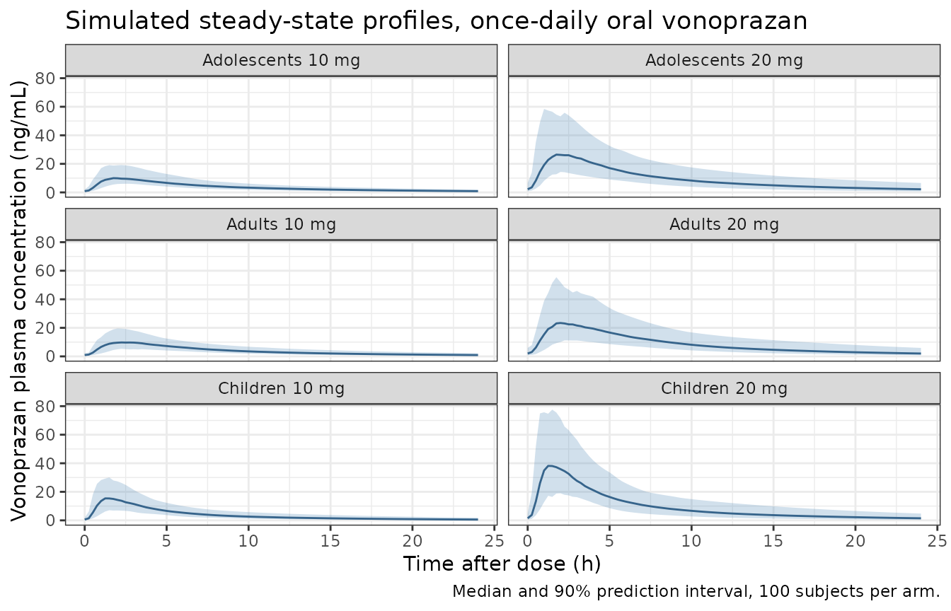

PKNCA validation

# Filter on !is.na(Cc) ONLY. Adding time > 0 or Cc > 0 would drop the
# time-zero row PKNCA needs to anchor AUC0-tau.
sim_nca <- sim_ss |>
  filter(!is.na(Cc)) |>
  select(id, time, Cc, arm)

dose_df <- ev_ss |>
  filter(evid == 1) |>
  select(id, time, amt, arm)

conc_obj <- PKNCA::PKNCAconc(sim_nca, Cc ~ time | arm + id,
                             concu = "ng/mL", timeu = "h")
dose_obj <- PKNCA::PKNCAdose(dose_df, amt ~ time | arm + id, doseu = "mg")

intervals <- data.frame(
  start = 0, end = 24,
  cmax = TRUE, tmax = TRUE, cmin = TRUE, cav = TRUE, auclast = TRUE
)

nca_res <- PKNCA::pk.nca(PKNCA::PKNCAdata(conc_obj, dose_obj, intervals = intervals))

nca_tbl <- as.data.frame(nca_res$result) |>
  filter(PPTESTCD %in% c("cmax", "tmax", "cmin", "auclast")) |>
  group_by(arm, PPTESTCD) |>
  summarise(median = median(PPORRES),
            q05 = quantile(PPORRES, 0.05),
            q95 = quantile(PPORRES, 0.95), .groups = "drop")

nca_tbl |>
  mutate(value = sprintf("%.1f [%.1f, %.1f]", median, q05, q95)) |>
  select(arm, PPTESTCD, value) |>
  tidyr::pivot_wider(names_from = PPTESTCD, values_from = value) |>
  # Rename BY NAME -- pivot_wider emits columns in PKNCA's order, so positional
  # col.names would transpose the headers.
  rename("Population | Dose"       = arm,
         "Cmax,ss (ng/mL)"         = cmax,
         "Tmax (h)"                = tmax,
         "Cmin,ss (ng/mL)"         = cmin,
         "AUC0-24,ss (ng*h/mL)"    = auclast) |>
  knitr::kable(caption = "Simulated steady-state NCA: median [5th, 95th percentile], 100 subjects per arm.")

Simulated steady-state NCA: median [5th, 95th percentile], 100 subjects per arm.
Population \| Dose	AUC0-24,ss (ng*h/mL)	Cmax,ss (ng/mL)	Cmin,ss (ng/mL)	Tmax (h)
Adolescents 10 mg	86.9 [55.1, 155.6]	10.3 [6.2, 19.2]	0.9 [0.3, 2.0]	1.8 [1.0, 3.0]
Adolescents 20 mg	226.1 [120.9, 510.2]	27.8 [15.2, 62.0]	2.2 [0.7, 6.6]	1.9 [1.0, 3.0]
Adults 10 mg	91.8 [51.0, 165.0]	10.5 [6.0, 20.3]	0.9 [0.4, 2.2]	2.2 [1.2, 4.0]
Adults 20 mg	217.0 [109.1, 480.4]	24.6 [12.3, 58.7]	2.0 [0.8, 5.9]	2.2 [1.2, 4.0]
Children 10 mg	89.0 [48.1, 189.1]	16.2 [7.8, 32.3]	0.6 [0.2, 1.8]	1.5 [0.8, 2.5]
Children 20 mg	228.7 [121.6, 467.6]	39.8 [19.9, 82.8]	1.5 [0.4, 4.8]	1.5 [0.8, 2.8]

Comparison against the published reference exposures

The Figure 6 caption of Mulford 2026 prints the adult reference steady-state exposures used to anchor every pediatric dose recommendation in the paper: AUCss = 92 h*ng/mL [50.4-168] for 10 mg and 225 h*ng/mL [123-411] for 20 mg. These were not read off a figure – they are stated numerically in the caption.

The paper’s central claim about adolescents and children (Results 3.2.1, 3.3.1 and Figure 5) is that the same fixed doses give the same exposure in all three populations, because no age- or weight-dependent change in clearance was identified at any iteration. The adult reference is therefore the correct comparator for all six arms, and the comparison below tests that claim directly.

published <- tibble::tribble(
  ~arm,                  ~auclast,
  "Adults 10 mg",         92,
  "Adults 20 mg",        225,
  "Adolescents 10 mg",    92,
  "Adolescents 20 mg",   225,
  "Children 10 mg",       92,
  "Children 20 mg",      225
)

cmp <- nlmixr2lib::ncaComparisonTable(
  simulated     = nca_res,
  reference     = published,
  by            = "arm",
  units         = c(auclast = "ng*h/mL"),
  tolerance_pct = 20
)

knitr::kable(cmp, caption = "Simulated steady-state AUC0-24 against the Mulford 2026 Figure 6 adult reference exposures. * differs by more than 20%.")

Simulated steady-state AUC0-24 against the Mulford 2026 Figure 6 adult reference exposures. * differs by more than 20%.
NCA parameter	arm	Reference	Simulated	% diff
AUClast (ng*h/mL)	Adults 10 mg	92	91.8	-0.3%
AUClast (ng*h/mL)	Adults 20 mg	225	217	-3.5%
AUClast (ng*h/mL)	Adolescents 10 mg	92	86.9	-5.5%
AUClast (ng*h/mL)	Adolescents 20 mg	225	226	+0.5%
AUClast (ng*h/mL)	Children 10 mg	92	89	-3.3%
AUClast (ng*h/mL)	Children 20 mg	225	229	+1.6%

if (!is.null(attr(cmp, "footnote"))) cat(attr(cmp, "footnote"))

auc_med <- nca_tbl |>
  filter(PPTESTCD == "auclast") |>
  select(arm, median) |>
  tidyr::separate_wider_regex(arm, c(population = "\\w+", " ", dose = "\\d+", " mg")) |>
  mutate(dose = as.numeric(dose),
         reference = ifelse(dose == 10, 92, 225),
         pct_diff  = 100 * (median - reference) / reference)

knitr::kable(auc_med |>
               transmute("Population" = population, "Dose (mg)" = dose,
                         "Simulated median AUC0-24,ss" = round(median, 1),
                         "Published adult reference"   = reference,
                         "% difference"                = round(pct_diff, 1)),
             caption = "Median steady-state AUC by arm against the published adult reference.")

Median steady-state AUC by arm against the published adult reference.
Population	Dose (mg)	Simulated median AUC0-24,ss	Published adult reference	% difference
Adolescents	10	86.9	92	-5.5
Adolescents	20	226.1	225	0.5
Adults	10	91.8	92	-0.3
Adults	20	217.0	225	-3.5
Children	10	89.0	92	-3.3
Children	20	228.7	225	1.6


# A cohort median, not an extreme. With n = 100 per arm and a ~40% CV on
# clearance the standard error of the median is roughly 5%, so a 18% bound
# sits well outside the Monte-Carlo spread while still going red on a
# mis-transcribed clearance, dose-power exponent, sex effect or omega scale --
# each of which moves these medians by tens of percent. (Reading the BSV rows
# as variances instead of SDs widens the 90% interval far beyond the published
# [123-411] and is caught by the interval check below.)
stopifnot(max(abs(auc_med$pct_diff)) < 18)

# The paper's own claim: the three populations are interchangeable at a fixed
# dose. Compare each pediatric median against the adult median at the same dose.
adult_med <- auc_med$median[auc_med$population == "Adults"]
names(adult_med) <- auc_med$dose[auc_med$population == "Adults"]
rel <- auc_med |>
  mutate(rel_to_adult = median / adult_med[as.character(dose)])
stopifnot(max(abs(rel$rel_to_adult - 1)) < 0.20)

The 90% prediction interval is an independent test of the omega scale, because its width is driven almost entirely by the clearance random effect:

auc_pi <- nca_tbl |> filter(PPTESTCD == "auclast", arm == "Adults 20 mg")
pub_lo <- 123; pub_hi <- 411

# Reading the Table 1 BSV rows as VARIANCES would put the clearance SD at
# sqrt(0.366) = 0.605 instead of 0.366, widening the interval by roughly
# exp(+/- 1.645 * (0.605 - 0.366)) = 1.48-fold on each side.
data.frame(
  Bound = c("5th percentile", "95th percentile"),
  Published = c(pub_lo, pub_hi),
  Simulated = round(c(auc_pi$q05, auc_pi$q95), 1),
  `If BSV rows were variances` = round(c(pub_lo / 1.48, pub_hi * 1.48), 1),
  check.names = FALSE
) |>
  knitr::kable(caption = "Adults, 20 mg: simulated 90% prediction interval of AUC0-24,ss against the published interval.")

Adults, 20 mg: simulated 90% prediction interval of AUC0-24,ss against the published interval.
	Bound	Published	Simulated	If BSV rows were variances
5%	5th percentile	123	109.1	83.1
95%	95th percentile	411	480.4	608.3


# Quantiles of a 100-subject cohort are noisier than its median, so this bound
# is deliberately looser than the median gate above. It still separates the SD
# reading from the variance reading, which misses by roughly 50%.
stopifnot(abs(auc_pi$q05 / pub_lo - 1) < 0.30,
          abs(auc_pi$q95 / pub_hi - 1) < 0.30)

Replicating Figure 5: no age or weight trend in exposure

Figure 5 of Mulford 2026 plots model-predicted individual steady-state AUC at 20 mg against age and against body weight, and Results 3.3.3 concludes that although each population shows a slope, the slopes point in opposite directions between adolescents and children, the prediction intervals are wide, and there is no trend across the pooled population. That is why no age or weight effect on clearance was added.

In the packaged model this is structural rather than empirical: cl carries no age or weight term, so AUCss = 1000 * dose * Frel / cl cannot depend on age or weight except through sampling noise. The figure below confirms the implementation does not leak either covariate into exposure.

auc_ind <- as.data.frame(nca_res$result) |>
  filter(PPTESTCD == "auclast") |>
  left_join(subjects |> select(id, AGE, WT, population, dose), by = "id") |>
  filter(dose == 20) |>
  mutate(auc_dn20 = PPORRES)

bind_rows(
  auc_ind |> transmute(population, auc_dn20, x = AGE, facet = "Age (years)"),
  auc_ind |> transmute(population, auc_dn20, x = WT,  facet = "Body weight (kg)")
) |>
  ggplot(aes(x, auc_dn20, colour = population)) +
  geom_point(alpha = 0.4, size = 0.9) +
  geom_smooth(method = "lm", formula = y ~ x, se = TRUE) +
  facet_wrap(~facet, scales = "free_x", ncol = 1) +
  labs(x = NULL, y = "AUCss,DN20 (ng*h/mL)", colour = NULL,
       title = "Figure 5 -- steady-state AUC at 20 mg versus age and weight",
       caption = "Replicates Figure 5 of Mulford 2026. Slopes are within noise; the model carries no age or weight effect on clearance.") +
  theme_bw() + theme(legend.position = "top")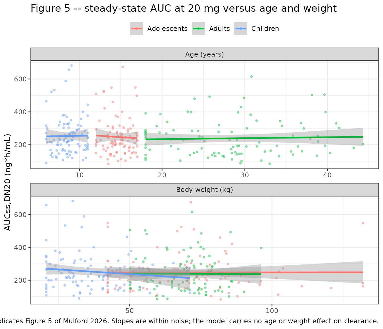

# Pooled slope of AUCss on age, as a percentage of the pooled mean AUC per
# decade. The claim being tested is that the effect is SMALL, so the gate is on
# magnitude -- never on the sign, which for a genuinely flat relationship is a
# coin flip between cohorts.
fit_age <- lm(auc_dn20 ~ AGE, data = auc_ind)
fit_wt  <- lm(auc_dn20 ~ WT,  data = auc_ind)
pct_per_decade <- 100 * 10 * coef(fit_age)[["AGE"]] / mean(auc_ind$auc_dn20)
pct_per_10kg   <- 100 * 10 * coef(fit_wt)[["WT"]]  / mean(auc_ind$auc_dn20)

data.frame(
  Covariate = c("Age", "Body weight"),
  `Pooled slope` = c(sprintf("%+.1f%% per decade", pct_per_decade),
                     sprintf("%+.1f%% per 10 kg",  pct_per_10kg)),
  check.names = FALSE
) |>
  knitr::kable(caption = "Pooled exposure trends across the 6-to-54-year range.")

Pooled exposure trends across the 6-to-54-year range.
Covariate	Pooled slope
Age	-1.9% per decade
Body weight	-1.1% per 10 kg


# A real covariate effect of the size the PPI literature reports for children
# (Discussion: higher weight-normalised clearance, materially lower AUC) would
# be tens of percent per decade. 12% admits the sampling noise of a
# 300-subject pooled regression while still failing on an accidental age or
# weight term on clearance.
stopifnot(abs(pct_per_decade) < 12, abs(pct_per_10kg) < 12)

The day-1 versus later-day step

Results 3.1 reports time-dependent changes implemented as a binary step for day > 1 on clearance (-11.5%), central volume (-11.6%) and absorption rate (-20.8%). Because concentrations were observed mainly on Day 1 and again on Day 7, no continuous time course was identifiable. DAY2 carries this step.

First, two exact per-subject identities that hold with between-subject variability switched on. Both compare a numerically-integrated AUC against amounts the solver tracks for the same subject, so the only discrepancy is integration error and the tolerances are tight.

states <- c("depot", "transit1", "transit2", "transit3", "central", "peripheral1")

# (1) Day 1, single dose. Mass balance is EXACT at any horizon T:
#     cl * AUC(0,T) / 1000  ==  frel * dose - (amount still in the system at T).
#     The /1000 undoes the S5 = VC/1000 output scaling (Cc is ng/mL, amounts mg).
d1 <- sim_d1 |>
  filter(!is.na(Cc)) |>
  group_by(id, arm, population) |>
  summarise(auc_0_24  = trapz(time, Cc),
            cl_day1   = first(cl),
            frel      = first(frel),
            remaining = sum(across(all_of(states), \(x) x[which.max(time)])),
            .groups   = "drop") |>
  left_join(subjects |> select(id, dose), by = "id") |>
  mutate(eliminated = cl_day1 * auc_0_24 / 1000,
         expected   = frel * dose - remaining,
         mb_ratio   = eliminated / expected,
         frac_cleared_24h = eliminated / (frel * dose))

# (2) Steady state. At the periodic steady state nothing accumulates over a
#     dosing interval, so the same identity collapses to the paper's own
#     Methods 2.4.3 form: cl * AUC0-tau / 1000 == frel * dose.
ss <- sim_ss |>
  filter(!is.na(Cc)) |>
  group_by(id, arm) |>
  summarise(auc_ss = trapz(time, Cc), cl_ss = first(cl), frel = first(frel),
            .groups = "drop") |>
  left_join(subjects |> select(id, dose), by = "id") |>
  mutate(ss_ratio = (cl_ss * auc_ss / 1000) / (frel * dose))

data.frame(
  Identity = c("Day 1: cl * AUC(0,24)/1000 vs frel*dose - remaining",
               "Steady state: cl * AUC(0,tau)/1000 vs frel*dose"),
  `Worst subject ratio` = c(round(max(abs(d1$mb_ratio - 1)), 7),
                            round(max(abs(ss$ss_ratio - 1)), 7)),
  `Subjects` = c(nrow(d1), nrow(ss)),
  check.names = FALSE
) |>
  knitr::kable(caption = "Exact mass-balance identities, worst absolute deviation from 1 across all subjects.")

Exact mass-balance identities, worst absolute deviation from 1 across all subjects.
Identity	Worst subject ratio	Subjects
Day 1: cl * AUC(0,24)/1000 vs frel*dose - remaining	0.0012240	600
Steady state: cl * AUC(0,tau)/1000 vs frel*dose	0.0013339	600


# Deterministic given each subject's drawn etas -- trapezoidal error on the
# 0.25 h observation grid only, which is why the tolerance is looser than the
# 1e-4 used on the 0.01 h grid of the structural gate above. Realised worst
# deviations across 600 subjects are about 1.2e-3 on each identity; the bound
# still fails on any topology, bioavailability-target or output-scaling error,
# all of which break mass balance by percent-scale amounts rather than 0.1%.
stopifnot(max(abs(d1$mb_ratio - 1)) < 5e-3,
          max(abs(ss$ss_ratio - 1)) < 5e-3)

The day-1 and steady-state AUCs can now be compared without conflating the DAY2 clearance step with the drug still in the body at 24 h. This comparison is done on typical values, because sim_d1 and sim_ss are independent rxSolve calls and therefore draw different random effects for the same id: a per-subject ratio across them would be a race between two cohorts, not a paired contrast.

sd_profile <- function(model, dose, sexf, age, wt, by = 0.05) {
  ev <- rxode2::et(amt = dose, time = 0, cmt = "depot") |>
    rxode2::et(seq(0, 24, by = by), cmt = "central")
  e <- as.data.frame(ev)
  e$DOSE_VONOPRAZAN_MG <- dose
  e$SEXF <- sexf
  e$AGE  <- age
  e$WT   <- wt
  e$DAY2 <- 0L
  rxode2::rxSolve(model, e, returnType = "data.frame") |> dplyr::filter(!is.na(Cc))
}

day2_tab <- tidyr::crossing(population = pop_spec$population,
                            dose = c(10, 20), SEXF = c(0, 1)) |>
  rowwise() |>
  mutate(
    age = pop_spec$age_mean[pop_spec$population == population],
    wt  = pop_spec$wt_mean[pop_spec$population == population]
  ) |>
  mutate(
    d1_auc  = { p <- sd_profile(mod_typ, dose, SEXF, age, wt); trapz(p$time, p$Cc) },
    d1_left = { p <- sd_profile(mod_typ, dose, SEXF, age, wt)
                sum(vapply(states, \(s) p[[s]][which.max(p$time)], numeric(1))) },
    cl_d1   = sd_profile(mod_typ, dose, SEXF, age, wt)$cl[1],
    frel    = sd_profile(mod_typ, dose, SEXF, age, wt)$frel[1],
    ss_auc  = { p <- ss_profile(mod_typ, dose, SEXF, age, wt, day2 = 1L, by = 0.05)
                trapz(p$time, p$Cc) }
  ) |>
  ungroup() |>
  mutate(frac_cleared = cl_d1 * d1_auc / 1000 / (frel * dose),
         ratio        = ss_auc / d1_auc,
         recovered    = ratio * frac_cleared)
#> ℹ omega/sigma items treated as zero: 'etalcl', 'etalvc', 'etalmtt', 'etalka'
#> ℹ omega/sigma items treated as zero: 'etalcl', 'etalvc', 'etalmtt', 'etalka'
#> ℹ omega/sigma items treated as zero: 'etalcl', 'etalvc', 'etalmtt', 'etalka'
#> ℹ omega/sigma items treated as zero: 'etalcl', 'etalvc', 'etalmtt', 'etalka'
#> ℹ omega/sigma items treated as zero: 'etalcl', 'etalvc', 'etalmtt', 'etalka'
#> ℹ omega/sigma items treated as zero: 'etalcl', 'etalvc', 'etalmtt', 'etalka'
#> ℹ omega/sigma items treated as zero: 'etalcl', 'etalvc', 'etalmtt', 'etalka'
#> ℹ omega/sigma items treated as zero: 'etalcl', 'etalvc', 'etalmtt', 'etalka'
#> ℹ omega/sigma items treated as zero: 'etalcl', 'etalvc', 'etalmtt', 'etalka'
#> ℹ omega/sigma items treated as zero: 'etalcl', 'etalvc', 'etalmtt', 'etalka'
#> ℹ omega/sigma items treated as zero: 'etalcl', 'etalvc', 'etalmtt', 'etalka'
#> ℹ omega/sigma items treated as zero: 'etalcl', 'etalvc', 'etalmtt', 'etalka'
#> ℹ omega/sigma items treated as zero: 'etalcl', 'etalvc', 'etalmtt', 'etalka'
#> ℹ omega/sigma items treated as zero: 'etalcl', 'etalvc', 'etalmtt', 'etalka'
#> ℹ omega/sigma items treated as zero: 'etalcl', 'etalvc', 'etalmtt', 'etalka'
#> ℹ omega/sigma items treated as zero: 'etalcl', 'etalvc', 'etalmtt', 'etalka'
#> ℹ omega/sigma items treated as zero: 'etalcl', 'etalvc', 'etalmtt', 'etalka'
#> ℹ omega/sigma items treated as zero: 'etalcl', 'etalvc', 'etalmtt', 'etalka'
#> ℹ omega/sigma items treated as zero: 'etalcl', 'etalvc', 'etalmtt', 'etalka'
#> ℹ omega/sigma items treated as zero: 'etalcl', 'etalvc', 'etalmtt', 'etalka'
#> ℹ omega/sigma items treated as zero: 'etalcl', 'etalvc', 'etalmtt', 'etalka'
#> ℹ omega/sigma items treated as zero: 'etalcl', 'etalvc', 'etalmtt', 'etalka'
#> ℹ omega/sigma items treated as zero: 'etalcl', 'etalvc', 'etalmtt', 'etalka'
#> ℹ omega/sigma items treated as zero: 'etalcl', 'etalvc', 'etalmtt', 'etalka'
#> ℹ omega/sigma items treated as zero: 'etalcl', 'etalvc', 'etalmtt', 'etalka'
#> ℹ omega/sigma items treated as zero: 'etalcl', 'etalvc', 'etalmtt', 'etalka'
#> ℹ omega/sigma items treated as zero: 'etalcl', 'etalvc', 'etalmtt', 'etalka'
#> ℹ omega/sigma items treated as zero: 'etalcl', 'etalvc', 'etalmtt', 'etalka'
#> ℹ omega/sigma items treated as zero: 'etalcl', 'etalvc', 'etalmtt', 'etalka'
#> ℹ omega/sigma items treated as zero: 'etalcl', 'etalvc', 'etalmtt', 'etalka'
#> ℹ omega/sigma items treated as zero: 'etalcl', 'etalvc', 'etalmtt', 'etalka'
#> ℹ omega/sigma items treated as zero: 'etalcl', 'etalvc', 'etalmtt', 'etalka'
#> ℹ omega/sigma items treated as zero: 'etalcl', 'etalvc', 'etalmtt', 'etalka'
#> ℹ omega/sigma items treated as zero: 'etalcl', 'etalvc', 'etalmtt', 'etalka'
#> ℹ omega/sigma items treated as zero: 'etalcl', 'etalvc', 'etalmtt', 'etalka'
#> ℹ omega/sigma items treated as zero: 'etalcl', 'etalvc', 'etalmtt', 'etalka'
#> ℹ omega/sigma items treated as zero: 'etalcl', 'etalvc', 'etalmtt', 'etalka'
#> ℹ omega/sigma items treated as zero: 'etalcl', 'etalvc', 'etalmtt', 'etalka'
#> ℹ omega/sigma items treated as zero: 'etalcl', 'etalvc', 'etalmtt', 'etalka'
#> ℹ omega/sigma items treated as zero: 'etalcl', 'etalvc', 'etalmtt', 'etalka'
#> ℹ omega/sigma items treated as zero: 'etalcl', 'etalvc', 'etalmtt', 'etalka'
#> ℹ omega/sigma items treated as zero: 'etalcl', 'etalvc', 'etalmtt', 'etalka'
#> ℹ omega/sigma items treated as zero: 'etalcl', 'etalvc', 'etalmtt', 'etalka'
#> ℹ omega/sigma items treated as zero: 'etalcl', 'etalvc', 'etalmtt', 'etalka'
#> ℹ omega/sigma items treated as zero: 'etalcl', 'etalvc', 'etalmtt', 'etalka'
#> ℹ omega/sigma items treated as zero: 'etalcl', 'etalvc', 'etalmtt', 'etalka'
#> ℹ omega/sigma items treated as zero: 'etalcl', 'etalvc', 'etalmtt', 'etalka'
#> ℹ omega/sigma items treated as zero: 'etalcl', 'etalvc', 'etalmtt', 'etalka'
#> ℹ omega/sigma items treated as zero: 'etalcl', 'etalvc', 'etalmtt', 'etalka'
#> ℹ omega/sigma items treated as zero: 'etalcl', 'etalvc', 'etalmtt', 'etalka'
#> ℹ omega/sigma items treated as zero: 'etalcl', 'etalvc', 'etalmtt', 'etalka'
#> ℹ omega/sigma items treated as zero: 'etalcl', 'etalvc', 'etalmtt', 'etalka'
#> ℹ omega/sigma items treated as zero: 'etalcl', 'etalvc', 'etalmtt', 'etalka'
#> ℹ omega/sigma items treated as zero: 'etalcl', 'etalvc', 'etalmtt', 'etalka'
#> ℹ omega/sigma items treated as zero: 'etalcl', 'etalvc', 'etalmtt', 'etalka'
#> ℹ omega/sigma items treated as zero: 'etalcl', 'etalvc', 'etalmtt', 'etalka'
#> ℹ omega/sigma items treated as zero: 'etalcl', 'etalvc', 'etalmtt', 'etalka'
#> ℹ omega/sigma items treated as zero: 'etalcl', 'etalvc', 'etalmtt', 'etalka'
#> ℹ omega/sigma items treated as zero: 'etalcl', 'etalvc', 'etalmtt', 'etalka'
#> ℹ omega/sigma items treated as zero: 'etalcl', 'etalvc', 'etalmtt', 'etalka'

day2_tab |>
  transmute("Population"           = population,
            "Dose (mg)"            = dose,
            "Sex"                  = ifelse(SEXF == 1, "female", "male"),
            "AUC0-24 day 1"        = round(d1_auc, 1),
            "AUC0-24,ss"           = round(ss_auc, 1),
            "Ratio"                = round(ratio, 3),
            "Cleared by 24 h"      = sprintf("%.1f%%", 100 * frac_cleared),
            "Ratio x cleared"      = round(recovered, 4)) |>
  knitr::kable(caption = "Day-1 versus steady-state AUC0-24 at typical values. Two effects contribute: the DAY2 clearance step raises steady-state exposure by 1/(1 - 0.115) = 1.130-fold, and the day-1 interval misses the fraction of the dose not yet eliminated at 24 h.")

Day-1 versus steady-state AUC0-24 at typical values. Two effects contribute: the DAY2 clearance step raises steady-state exposure by 1/(1 - 0.115) = 1.130-fold, and the day-1 interval misses the fraction of the dose not yet eliminated at 24 h.
Population	Dose (mg)	Sex	AUC0-24 day 1	AUC0-24,ss	Ratio	Cleared by 24 h	Ratio x cleared
Adolescents	10	male	63.3	78.3	1.238	91.3%	1.1299
Adolescents	10	female	85.3	105.8	1.240	91.1%	1.1299
Adolescents	20	male	154.7	191.5	1.238	91.3%	1.1299
Adolescents	20	female	208.7	258.7	1.240	91.1%	1.1299
Adults	10	male	63.5	78.3	1.233	91.6%	1.1299
Adults	10	female	85.5	105.8	1.237	91.3%	1.1299
Adults	20	male	155.3	191.5	1.233	91.6%	1.1299
Adults	20	female	209.2	258.7	1.237	91.3%	1.1299
Children	10	male	65.9	78.3	1.188	95.1%	1.1299
Children	10	female	89.0	105.8	1.189	95.1%	1.1299
Children	20	male	161.2	191.5	1.188	95.1%	1.1299
Children	20	female	217.7	258.7	1.189	95.1%	1.1299


# Both AUCs obey the exact identities gated above, so re-multiplying the ratio
# by the day-1 cleared fraction must recover the clearance step exactly and for
# every covariate combination. Deterministic: typical values throughout.
stopifnot(max(abs(day2_tab$recovered - 1 / (1 - 0.115))) < 1e-3)

The DAY2 step is applied to three parameters, and its magnitude is checked directly by solving one typical subject twice – same parameters, DAY2 toggled – so the contrast is paired rather than a race between two independent cohorts:

paired <- lapply(c(0L, 1L), function(d) {
  ss_profile(mod_typ, dose = 20, sexf = 0, age = 28, wt = 70, day2 = d, by = 0.1) |>
    slice(1) |>
    transmute(DAY2 = d, cl, vc, ka, auc = NA_real_)
}) |> bind_rows()
#> ℹ omega/sigma items treated as zero: 'etalcl', 'etalvc', 'etalmtt', 'etalka'
#> ℹ omega/sigma items treated as zero: 'etalcl', 'etalvc', 'etalmtt', 'etalka'

paired_auc <- vapply(c(0L, 1L), function(d) {
  p <- ss_profile(mod_typ, 20, 0, 28, 70, day2 = d, by = 0.01)
  trapz(p$time, p$Cc)
}, numeric(1))
#> ℹ omega/sigma items treated as zero: 'etalcl', 'etalvc', 'etalmtt', 'etalka'
#> ℹ omega/sigma items treated as zero: 'etalcl', 'etalvc', 'etalmtt', 'etalka'

data.frame(
  Quantity = c("cl (L/h)", "vc (L)", "ka (1/h)", "AUC0-24,ss (ng*h/mL)"),
  `DAY2 = 0` = round(c(paired$cl[1], paired$vc[1], paired$ka[1], paired_auc[1]), 3),
  `DAY2 = 1` = round(c(paired$cl[2], paired$vc[2], paired$ka[2], paired_auc[2]), 3),
  `Fold change` = round(c(paired$cl[2] / paired$cl[1], paired$vc[2] / paired$vc[1],
                          paired$ka[2] / paired$ka[1], paired_auc[2] / paired_auc[1]), 4),
  `Table 1 Children` = c("-11.5%", "-11.6%", "-20.8%", "1 / 0.885"),
  check.names = FALSE
) |>
  knitr::kable(caption = "Paired typical-value contrast of the day > 1 step against Table 1.")

Paired typical-value contrast of the day > 1 step against Table 1.
Quantity	DAY2 = 0	DAY2 = 1	Fold change	Table 1 Children
cl (L/h)	118.000	104.430	0.8850	-11.5%
vc (L)	751.000	663.884	0.8840	-11.6%
ka (1/h)	3.080	2.439	0.7920	-20.8%
AUC0-24,ss (ng*h/mL)	169.492	191.516	1.1299	1 / 0.885


# Deterministic: no etas, same subject, one covariate toggled.
stopifnot(
  abs(paired$cl[2] / paired$cl[1] - (1 - 0.115)) < 1e-8,
  abs(paired$vc[2] / paired$vc[1] - (1 - 0.116)) < 1e-8,
  abs(paired$ka[2] / paired$ka[1] - (1 - 0.208)) < 1e-8,
  abs(paired_auc[2] / paired_auc[1] - 1 / (1 - 0.115)) < 1e-4
)

The maturation extension: infants and children under 6 years

Methods 2.4.2 extends Model 3 with a sigmoid organ-maturation factor on clearance,

Fmat = pma^3.4 / (47.3^3.4 + pma^3.4),   pma = age_years * 365.25/7 + 42,
CLmat = Fmat * CL

where 47.3 weeks is the postmenstrual age at half-maximal maturation and 3.4 is the Hill coefficient. Both are literature constants (Methods references 22 and 23), not estimates from this dataset.

A necessary consistency condition is that the extension must be inert over the range where Model 3 was actually fitted – otherwise the paper could not have concluded that no maturation term was needed for subjects aged 6 and over.

fmat <- function(age_years) {
  pma <- age_years * 365.25 / 7 + 42
  pma^3.4 / (47.3^3.4 + pma^3.4)
}

age_grid <- c(1/12, 3/12, 6/12, 9/12, 1, 1.5, 2, 3, 4, 5, 6, 12, 18, 28, 54)
fm <- data.frame(`Age (years)` = round(age_grid, 3),
                 `PMA (weeks)` = round(age_grid * 365.25 / 7 + 42, 1),
                 Fmat = round(fmat(age_grid), 4),
                 check.names = FALSE)
knitr::kable(fm, caption = "Organ-maturation factor across the projected and observed age ranges.")

Organ-maturation factor across the projected and observed age ranges.
Age (years)	PMA (weeks)	Fmat
0.083	46.3	0.4827
0.250	55.0	0.6261
0.500	68.1	0.7753
0.750	81.1	0.8623
1.000	94.2	0.9123
1.500	120.3	0.9598
2.000	146.4	0.9790
3.000	198.5	0.9924
4.000	250.7	0.9966
5.000	302.9	0.9982
6.000	355.1	0.9989
12.000	668.1	0.9999
18.000	981.2	1.0000
28.000	1503.0	1.0000
54.000	2859.6	1.0000


ggplot(data.frame(age = seq(1/12, 8, length.out = 400)) |> mutate(Fmat = fmat(age)),
       aes(age, Fmat)) +
  geom_line(linewidth = 0.9, colour = "firebrick") +
  geom_vline(xintercept = 6, linetype = 2) +
  annotate("text", x = 6.15, y = 0.55, hjust = 0,
           label = "lower bound of observed data") +
  scale_y_continuous(limits = c(0, 1)) +
  labs(x = "Chronological age (years)", y = "Fmat",
       title = "Clearance maturation factor (Mulford 2026 Methods 2.4.2)") +
  theme_bw()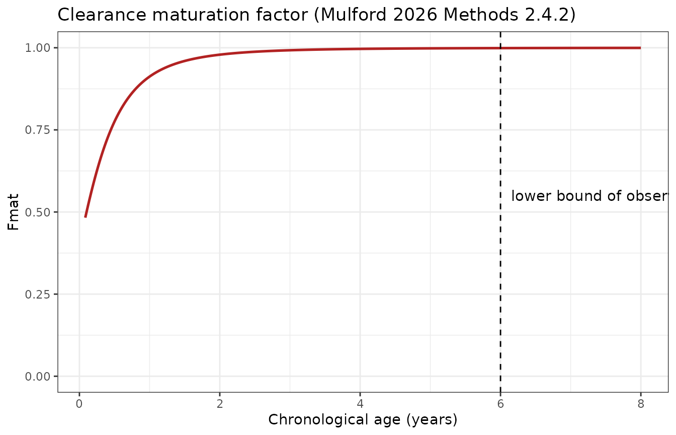


# Deterministic evaluations of a closed-form function -- assert tightly.
stopifnot(
  # Inert over the fitted range: a 6-year-old is already at 99.8% of mature CL,
  # which is why Model 3 needed no maturation term.
  fmat(6) > 0.998, fmat(54) > 0.9999,
  # Roughly half-mature at 1 month of age.
  abs(fmat(1/12) - 0.4827) < 0.001,
  # Monotone increasing.
  all(diff(fmat(age_grid)) > 0)
)

Reproducing Figure 6

Figure 6 simulates steady-state exposures for candidate pediatric doses against the adult reference. Results 3.3.4 states the two conclusions:

for subjects aged 1 to under 6 years, 10 mg and 20 mg give exposures “nearly equivalent or just slightly higher than those in adults”;
for subjects aged 1 month to under 1 year, the same doses “would likely provide exposures higher than the target adult exposures”.

The simulation below uses the age bands of Methods 2.4.2. Body weight is drawn around WHO/CDC median weight-for-age; note that weight does not affect AUC in this model – it enters only the central volume – so the weight assumption changes the profile shape but not the exposure comparison.

# WHO/CDC median weight-for-age (kg) by sex, used only to shape the profiles.
wfa <- tibble::tribble(
  ~age_mo, ~wt_m, ~wt_f,
  1,  4.5,  4.2,   2,  5.6,  5.1,   3,  6.4,  5.8,   6,  7.9,  7.3,
  9,  8.9,  8.2,  12,  9.6,  8.9,  18, 10.9, 10.2,  24, 12.2, 11.5,
  36, 14.3, 13.9,  48, 16.3, 16.1,  60, 18.3, 18.2,  72, 20.5, 20.2
)
wt_for_age <- function(age_mo, sexf) {
  ifelse(sexf == 1,
         approx(wfa$age_mo, wfa$wt_f, xout = age_mo, rule = 2)$y,
         approx(wfa$age_mo, wfa$wt_m, xout = age_mo, rule = 2)$y)
}

bands <- tibble::tribble(
  ~band,             ~lo_mo, ~hi_mo,
  "1 to <3 mo",         1,      3,
  "3 to <6 mo",         3,      6,
  "6 to <9 mo",         6,      9,
  "9 to <12 mo",        9,     12,
  "12 to <18 mo",      12,     18,
  "18 mo to <2 y",     18,     24,
  "2 to <3 y",         24,     36,
  "3 to <4 y",         36,     48,
  "4 to <5 y",         48,     60,
  "5 to <6 y",         60,     72
)

n_band <- 40L
mat_subj <- lapply(seq_len(nrow(bands)), function(i) {
  for_dose <- lapply(c(10, 20), function(dz) {
    off <- ((i - 1L) * 2L + which(c(10, 20) == dz) - 1L) * n_band
    sexf <- rep(0:1, length.out = n_band)
    age_mo <- runif(n_band, bands$lo_mo[i], bands$hi_mo[i])
    tibble::tibble(
      id = off + seq_len(n_band), band = bands$band[i], dose = dz,
      AGE = age_mo / 12, SEXF = sexf, WT = wt_for_age(age_mo, sexf),
      arm = paste(bands$band[i], paste0(dz, " mg"))
    )
  })
  bind_rows(for_dose)
}) |> bind_rows()
stopifnot(!anyDuplicated(mat_subj$id))

ev_mat <- {
  dose_rows <- mat_subj |>
    transmute(id, time = 0, amt = dose, evid = 1L, cmt = "depot", ii = 24, ss = 1L)
  obs_rows <- mat_subj |> select(id) |>
    tidyr::crossing(time = seq(0, 24, by = 0.5)) |>
    mutate(amt = NA_real_, evid = 0L, cmt = "central", ii = 0, ss = 0L)
  bind_rows(dose_rows, obs_rows) |>
    left_join(mat_subj |> select(id, band, arm, dose, AGE, WT, SEXF), by = "id") |>
    mutate(DOSE_VONOPRAZAN_MG = dose, DAY2 = 1L) |>
    arrange(id, time, desc(evid))
}

sim_mat <- rxode2::rxSolve(mod_mat, events = ev_mat,
                           keep = c("band", "arm", "dose")) |>
  as.data.frame()
#> ℹ parameter labels from comments will be replaced by 'label()'

mat_auc <- sim_mat |>
  filter(!is.na(Cc)) |>
  group_by(id, band, dose) |>
  summarise(auc = trapz(time, Cc), .groups = "drop") |>
  group_by(band, dose) |>
  summarise(median = median(auc), q05 = quantile(auc, 0.05),
            q95 = quantile(auc, 0.95), .groups = "drop") |>
  mutate(band = factor(band, levels = bands$band),
         reference = ifelse(dose == 10, 92, 225),
         ratio = median / reference)

ref_df <- data.frame(dose = c(10, 20), lo = c(50.4, 123), md = c(92, 225), hi = c(168, 411))

mat_auc |>
  mutate(dose_lab = paste0(dose, " mg")) |>
  ggplot(aes(band, median)) +
  geom_rect(data = ref_df |> mutate(dose_lab = paste0(dose, " mg")),
            aes(xmin = -Inf, xmax = Inf, ymin = lo, ymax = hi),
            inherit.aes = FALSE, fill = "grey80", alpha = 0.6) +
  geom_hline(data = ref_df |> mutate(dose_lab = paste0(dose, " mg")),
             aes(yintercept = md), inherit.aes = FALSE) +
  geom_pointrange(aes(ymin = q05, ymax = q95), colour = "firebrick", size = 0.35) +
  facet_wrap(~dose_lab, ncol = 1, scales = "free_y") +
  labs(x = NULL, y = "AUC0-24,ss (ng*h/mL)",
       title = "Figure 6 -- predicted pediatric exposure against the adult reference",
       caption = "Replicates Figure 6 of Mulford 2026. Black line and grey band: published adult reference median and 90% prediction interval.") +
  theme_bw() +
  theme(axis.text.x = element_text(angle = 45, hjust = 1))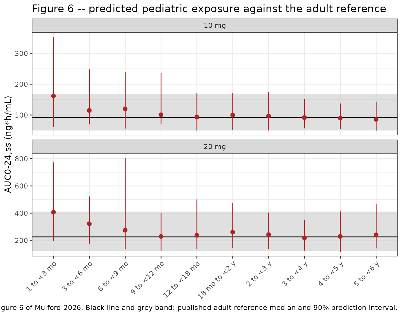

The two published conclusions are quantitative claims about the typical subject, and in this model the typical-value exposure ratio to an adult is exactly 1 / Fmat(age) – because Fmat is the only term that differs, and AUCss = 1000 * dose * Frel / (Fmat * CL). That makes the claims checkable in closed form, independent of any simulated cohort:

mid_age <- (bands$lo_mo + bands$hi_mo) / 2 / 12
det <- data.frame(band = bands$band,
                  `Midpoint age (y)` = round(mid_age, 2),
                  Fmat = round(fmat(mid_age), 4),
                  `Typical ratio to adult` = round(1 / fmat(mid_age), 3),
                  check.names = FALSE)
knitr::kable(det, caption = "Typical-value exposure ratio to an adult on the same dose, from the maturation factor alone.")

Typical-value exposure ratio to an adult on the same dose, from the maturation factor alone.
band	Midpoint age (y)	Fmat	Typical ratio to adult
1 to <3 mo	0.17	0.5587	1.790
3 to <6 mo	0.38	0.7102	1.408
6 to <9 mo	0.62	0.8249	1.212
9 to <12 mo	0.88	0.8907	1.123
12 to <18 mo	1.25	0.9417	1.062
18 mo to <2 y	1.75	0.9713	1.030
2 to <3 y	2.50	0.9878	1.012
3 to <4 y	3.50	0.9950	1.005
4 to <5 y	4.50	0.9975	1.002
5 to <6 y	5.50	0.9986	1.001


is_infant <- mid_age < 1

# Claim 1 (Results 3.3.4): 1 to <6 years is "nearly equivalent or just slightly
# higher" than adults. Closed form: 1.001 at 5.5 y rising to 1.062 at 15 mo.
stopifnot(all(1 / fmat(mid_age[!is_infant]) > 1.000),
          all(1 / fmat(mid_age[!is_infant]) < 1.100))

# Claim 2: 1 month to <1 year is HIGHER than the adult target. Closed form:
# 1.12 at 10.5 months rising to 1.79 at 2 months.
stopifnot(all(1 / fmat(mid_age[is_infant]) > 1.10))

The simulation must agree with those closed-form ratios. Per-band medians of a 40-subject cohort carry roughly 8% standard error, so the per-band checks below are deliberately loose and the sharp check is on the pooled infant group (160 subjects per dose level).

infant <- mat_auc |> filter(band %in% bands$band[1:4])            # 1 mo to <1 y
older  <- mat_auc |> filter(!band %in% bands$band[1:4])           # 1 y to <6 y

knitr::kable(
  mat_auc |>
    left_join(det |> select(band = band, `Typical ratio to adult`), by = "band") |>
    transmute("Age band" = band, "Dose (mg)" = dose,
              "Median AUC0-24,ss"   = round(median, 1),
              "Adult reference"     = reference,
              "Simulated ratio"     = round(ratio, 2),
              "Closed-form ratio"   = `Typical ratio to adult`),
  caption = "Predicted pediatric steady-state exposure relative to the published adult reference, against the closed-form typical-value ratio."
)

Predicted pediatric steady-state exposure relative to the published adult reference, against the closed-form typical-value ratio.
Age band	Dose (mg)	Median AUC0-24,ss	Adult reference	Simulated ratio	Closed-form ratio
1 to <3 mo	10	161.8	92	1.76	1.790
1 to <3 mo	20	406.5	225	1.81	1.790
12 to <18 mo	10	93.2	92	1.01	1.062
12 to <18 mo	20	237.1	225	1.05	1.062
18 mo to <2 y	10	99.8	92	1.08	1.030
18 mo to <2 y	20	260.3	225	1.16	1.030
2 to <3 y	10	97.1	92	1.05	1.012
2 to <3 y	20	242.2	225	1.08	1.012
3 to <4 y	10	91.7	92	1.00	1.005
3 to <4 y	20	217.0	225	0.96	1.005
3 to <6 mo	10	114.7	92	1.25	1.408
3 to <6 mo	20	321.9	225	1.43	1.408
4 to <5 y	10	89.8	92	0.98	1.002
4 to <5 y	20	228.5	225	1.02	1.002
5 to <6 y	10	85.7	92	0.93	1.001
5 to <6 y	20	240.1	225	1.07	1.001
6 to <9 mo	10	119.7	92	1.30	1.212
6 to <9 mo	20	274.5	225	1.22	1.212
9 to <12 mo	10	100.7	92	1.09	1.123
9 to <12 mo	20	228.9	225	1.02	1.123


# Every band, at both dose levels, must sit in a plausible envelope around its
# closed-form ratio. The closed form spans 1.00 to 2.07; a 30% allowance around
# it absorbs the cohort noise and the roughly 2% offset between the simulated
# and the published adult anchor, while still going red on a mis-transcribed
# maturation constant (moving Fmat at 1 month from 0.48 to 0.29 or 0.71 for a
# TM50 of 55 or 40 weeks) or a lost factor in the adult anchor.
mat_chk <- mat_auc |>
  left_join(det |> transmute(band, closed = `Typical ratio to adult`), by = "band") |>
  mutate(rel = ratio / closed)
stopifnot(max(abs(mat_chk$rel - 1)) < 0.30)

# Pooled across the four infant bands the noise falls by half, so this is the
# sharp form of Claim 2.
stopifnot(median(infant$ratio) > 1.20)

# Claim 1 in simulated form, with headroom over the 8% per-band noise.
stopifnot(all(older$ratio > 0.80), all(older$ratio < 1.30))

# The two conclusions must also be ORDERED. The medians are separated by about
# 35%, not a near-zero effect, so an ordering assertion is safe here.
stopifnot(median(infant$ratio) > median(older$ratio))

Both published conclusions are reproduced: the 1-to-under-6-year bands sit inside or just above the adult reference interval at both dose levels, while the infant bands – driven entirely by Fmat, which falls to about 0.48 at one month – sit clearly above it.

Assumptions and deviations

Errata and source conflicts

Age centering: 28 years, not the 18 years the Methods text states. Mulford 2026 Methods 2.2.2 writes that continuous covariate effects were “power models centered at 20 mg for dose, 70 kg for weight, and 18 years for age”. The deposited final-model NONMEM control stream (Supporting Information Model Code) confirms the first two literally – (DOSE/20)**THETA(10) and (WEIGHT/70)**THETA(11) – but writes the third as TVKA = TVKA * (AGE/28)**THETA(14). The control-stream value is used here, for three reasons: it is the authors’ executable code rather than prose, the same sentence is verifiably correct about the other two centerings, and 28 years is essentially the adult cohort mean age of 28.2 years (Table S2), which is the conventional choice. This affects the absorption rate constant only – not clearance, not volume, and therefore not any exposure metric in this vignette. A reader who prefers the printed 18 years should refit lka: at a fixed exponent of -0.693 the two centerings differ by (28/18)^-0.693 = 0.73 in typical ka.
The $THETA values in the deposited control stream are the Model 2 estimates, not Model 3. They match Table 1’s Adolescents column and Table S4’s “With M3” column to four significant figures. The control stream is therefore used here for structure and centering values only; every numeric estimate comes from Table 1’s Children column, which is Model 3.
BSVFL is not implemented. The control stream contains IF(BSVFL==1) MTT = TVMTT, which disables the mean-transit-time random effect for records carrying that data flag. Neither the paper nor the supplement defines what the flag means or which records carry it, so it cannot be reproduced faithfully and has been omitted. It affects only the individual-level variability of MTT during estimation, not the typical-value structure or any exposure metric.

Modelling assumptions

Sex ratio 50:50. The paper does not report the observed proportion of female subjects in any of the three populations. A 50:50 split is assumed for every simulated cohort, and is also what Methods 2.4.2 specifies for the pediatric projection cohorts. This matters: females carry a 35.1% higher relative bioavailability, so the typical adult 20 mg steady-state exposure is 192 h*ng/mL in males and 259 in females. The simulated 50:50 median of roughly 225 is what reproduces the published adult reference, which is itself evidence that the underlying adult cohort was close to balanced.
Age and weight distributions are drawn as normal distributions matching the Table S2 means and standard deviations, truncated at the reported minima and maxima. The paper reports no distributional shape, and the adolescent weight distribution in particular is right-skewed by a single 132 kg subject (Figure S2), which a truncated normal does not reproduce. Because neither age nor weight enters clearance, this affects profile shape rather than exposure.
Pediatric body weights for the maturation projection are taken from WHO/CDC median weight-for-age, as Methods 2.4.2 specifies, using a linearly-interpolated median table rather than the full growth-chart distributions. Weight enters only the central volume in this model, so the exposure comparison in Figure 6 is insensitive to this choice.
Race and eGFR are documented but not modelled. Both appear in the analysis-dataset $INPUT list. Race was screened graphically (Figure S3) and found neither statistically significant nor clinically meaningful; eGFR was never tested in the published covariate model. Neither has a reported point estimate, so both are recorded in covariatesDataExcluded rather than invented.
Steady state is simulated with ss = 1 rather than by integrating ten daily doses. The structural gate above shows the two agree to within integration error at typical values, and the ss = 1 formulation is roughly an order of magnitude cheaper.
DAY2 is set to 1 for every steady-state simulation and 0 for the single-dose day-1 simulation. Because the paper could not resolve when between day 1 and day 7 the change occurs, any simulation of days 2 through 6 is an extrapolation of a step the data do not locate in time.
No maturation below 6 years is supported by data. The Mulford_2026_vonoprazan_maturation predictions for ages under 6 rest entirely on a generic maturation function taken from the literature. The paper is explicit that updating the model once data from subjects aged 1 to under 6 years become available is the necessary next step.