Prednisolone (Mohlmann 2026)
Source:vignettes/articles/Mohlmann_2026_prednisolone.Rmd
Mohlmann_2026_prednisolone.RmdModel and source
#> ℹ parameter labels from comments will be replaced by 'label()'Citation: Mohlmann JE, Lindemans CA, Jansen MHA, van Luin M, Punt AM, Ezzafzafi S, Nierkens S, Huitema ADR, de Vries Schultink AHM. Population Pharmacokinetics of Total and Protein-Unbound Prednisolone in Children with Immune-Mediated and Systemic Inflammatory Diseases. Clin Pharmacokinet. 2026;65(3):277-292. doi:10.1007/s40262-025-01601-5
Description: Two-compartment population PK model for total and protein-unbound prednisolone in children with immune-mediated and systemic inflammatory diseases, oral or IV (Mohlmann 2026). First-order absorption with F fixed to 1; the disposition is parameterised on UNBOUND prednisolone with allometric scaling to 70 kg (exponents fixed at 0.75 and 1). Total prednisolone is recovered algebraically from linear binding to albumin plus saturable binding to corticosteroid-binding globulin (transcortin), the latter supplied as a time-varying covariate that follows its circadian rhythm. Clearance differs by cohort (HCT prophylaxis, HCT GvHD therapy, autoimmune disease as reference).
Article: https://doi.org/10.1007/s40262-025-01601-5 (open access, https://europepmc.org/article/PMC/PMC12881105)
Online Resource 3 of the electronic supplementary material prints the final NONMEM control stream. Every parameter value in the model comes from that control stream; Table 2 of the article prints the same estimates, rounded.
Population
Sixty children and young adults from two prospective studies at the University Medical Centre Utrecht (Methods 2.1-2.2, Table 1, Table S1): 44 after allogeneic haematopoietic cell transplantation (HCT, PIKACHU study), receiving prednisolone either as GvHD prophylaxis (1 mg/kg/day IV in two doses after a cord-blood transplant) or as therapy of GvHD or engraftment syndrome (2 mg/kg/day), and 16 with autoimmune or systemic inflammatory disease (SLE, uveitis, IBD and others; CARPE DIEM study) taking oral prednisolone, usually once daily. Median age 10 years (range 0.2-19), median weight 36.5 kg (5.0-109), 43% female. The PK dose was a median 0.5 mg/kg (0.25-1); 66% of the 68 PK occasions were IV. Median albumin was 31.1 g/L and median measured corticosteroid-binding globulin (CBG) 1.09 umol/L. In total 305 total and 304 unbound (equilibrium dialysis) serum prednisolone concentrations were measured.
Model structure
The disposition is a two-compartment model with first-order
absorption, and both ODE states hold unbound
prednisolone: CL and Q act on the unbound pool, and the control stream
reads the unbound concentration directly off the central compartment
(CPU = A(2)/S2). The total concentration is an output
transformation (Eqs 1-2; control stream CP):
with all concentrations in umol/L. Binding moves no mass and never
feeds back on the disposition. Following the library convention,
Cc is the central-pool (unbound) concentration and
Ctot the total.
Three unit conversions come straight from the control stream:
prednisolone mg/L to umol/L by 2.77 (S2 = V2/2.77, MW
360.4), albumin g/L to umol/L by dividing by 0.0665
(ALBX = ALBM/0.0665), and CBG mg/L to umol/L by dividing by
52 (52 kDa, Discussion 4.3).
CBG is a time-varying covariate. CBG was measured
once per occasion; the authors then used the circadian model of Melin et
al. (Eqs 7-8) to estimate each child’s full 24-h CBG curve and supplied
it to NONMEM as a data column. The model therefore reads
TRANSCORTIN (mg/L) at every record rather than computing
the rhythm itself. The helper below rebuilds the curve from a baseline
value with Eqs 7-8; TIME there is hours after 3 PM.
# Eqs 7-8: CBGt = CBGb * (1 + Circ), with
# Circ = AMP24 cos(2 pi (TIME - SHIFT24) / 24) + AMP12 cos(2 pi (TIME - SHIFT12) / 12)
# AMP24 0.055, SHIFT24 1.8 h, AMP12 0.029, SHIFT12 15.7 h; TIME in h after 3 PM.
cbg_curve_um <- function(clock_h, cbg_base_um) {
  t_3pm <- (clock_h - 15) %% 24
  circ <- 0.055 * cos(2 * pi * (t_3pm - 1.8) / 24) +
    0.029 * cos(2 * pi * (t_3pm - 15.7) / 12)
  cbg_base_um * (1 + circ)
}
mw_cbg_kda <- 52 # converts umol/L to mg/L
The cohort covariate on CL has three levels (control-stream
PorT): HCT prophylaxis (x 1.10), HCT GvHD therapy (x 0.975)
and autoimmune disease (the reference). It is encoded with two
indicators, TX_HCT (1 for both HCT levels) and
AGVHD_ANY (1 for the GvHD-therapy level), so that
hct_proph = TX_HCT * (1 - AGVHD_ANY) and
hct_ther = TX_HCT * AGVHD_ANY reproduce
THETA(8)**PP * THETA(9)**PT.
Source trace
| Quantity | Value | Source |
|---|---|---|
| ka | 0.68 1/h | Online Resource 3 THETA(1); Table 2 |
| CL (70 kg, autoimmune) | 155 L/h | THETA(2); Table 2 |
| Vc (70 kg) | 338 L | THETA(3); Table 2 |
| Q (70 kg) | 105 L/h | THETA(4); Table 2 |
| Vp (70 kg) | 170 L | THETA(5); Table 2 |
| Kalb | 200 umol/L | THETA(6); Table 2 |
| KCBG | 0.0476 umol/L | THETA(7); Results 3.4 (Table 2 rounds to 0.048) |
| HCT-prophylaxis on CL | 1.1 | THETA(8); Table 2 1.10 |
| HCT-therapy on CL | 0.975 | THETA(9); Table 2 0.97 |
| Allometric exponents | 0.75 (CL, Q), 1 (Vc, Vp), fixed | Methods 2.4.1; $PK; Results 3.3 |
| F | 1, fixed | Results 3.3; no F in $PK
|
| IIV CL, Vc, Vp (block) | 0.0993, 0.365, 0.153; cov 0.097 (CL-Vc), -0.14 (Vc-Vp), 0 (CL-Vp) |
$OMEGA BLOCK(3); Table 2 |
| IIV ka | 0.268 |
$OMEGA; Table 2 |
| Proportional error, unbound | variance 0.114 |
$SIGMA; Table 2 33.8% |
| Proportional error, total | variance 0.0703 |
$SIGMA; Table 2 26.5% |
| Binding equation | Eqs 1-2 | Methods 2.4.1; $ERROR CP
|
| Unit conversions 2.77, 0.0665, 52 | – |
$PK S2, ALBX; Discussion
4.3 |
| CBG circadian curve | Eqs 7-8 | Methods 2.4.3 |
Omega and sigma scale
The control stream carries variances and Table 2 prints the square root as a percentage. Recomputing every Table 2 entry from the variances confirms the scale:
om <- c(cl = 0.0993, vc = 0.365, vp = 0.153, ka = 0.268)
check <- data.frame(
  Quantity = c("IIV CL", "IIV Vc", "IIV Vp", "IIV ka", "Corr CL-Vc", "Corr Vc-Vp",
               "Prop. error unbound", "Prop. error total"),
  Recomputed = 100 * c(
    sqrt(om), 0.097 / sqrt(om[["cl"]] * om[["vc"]]),
    -0.14 / sqrt(om[["vc"]] * om[["vp"]]), sqrt(0.114), sqrt(0.0703)
  ),
  Table2 = c(31.5, 60.4, 39.1, 51.8, 51.0, -59.0, 33.8, 26.5)
)
check$Recomputed <- round(check$Recomputed, 1)
knitr::kable(check, caption = "Table 2 percentages recomputed from the control-stream variances.")| Quantity | Recomputed | Table2 |
|---|---|---|
| IIV CL | 31.5 | 31.5 |
| IIV Vc | 60.4 | 60.4 |
| IIV Vp | 39.1 | 39.1 |
| IIV ka | 51.8 | 51.8 |
| Corr CL-Vc | 51.0 | 51.0 |
| Corr Vc-Vp | -59.2 | -59.0 |
| Prop. error unbound | 33.8 | 33.8 |
| Prop. error total | 26.5 | 26.5 |
# The variances round to Table 2 exactly. The correlations differ by up to 0.2
# points because the control stream prints the covariances to two or three
# significant figures (0.097, -0.14); a variance-vs-SD mix-up would be off by
# tens of points.
stopifnot(all(abs(check$Recomputed - check$Table2) < 0.25))
Typical-patient simulations (Figure 7)
Section 2.6 describes the simulated typical patient: 30 kg,
prednisolone 0.5 mg/kg IV twice daily, baseline CBG 1.0 umol/L, albumin
35 g/L, typical parameters. The IV dose is prednisolone sodium
succinate, and the data column AMT is the salt-corrected
amount, so a 15 mg IV dose enters the model as 15 x 0.75 = 11.25 mg of
prednisolone. The paper does not say when the doses were given; 8 AM and
8 PM are assumed here. Unless stated otherwise the patient is in the
autoimmune (reference) cohort.
mod_typ <- rxode2::zeroRe(mod)

# One-subject typical-value solve. `clock0` is the clock hour at time 0, so the
# CBG curve is evaluated on the clock. Observation rows sit on the ODE state
# `central` with dvid = 1; rxSolve returns both Cc and Ctot as columns.
sim_typ <- function(dose_times, amt, cmt = "central", wt = 30, cbg_base = 1.0,
                    tx_hct = 0, agvhd = 0, t_end = 24, etalcl = 0, clock0 = 0) {
  obs_t <- seq(0, t_end, by = 0.02)
  ev <- dplyr::bind_rows(
    data.frame(time = dose_times, amt = amt, cmt = cmt, evid = 1L, dvid = NA_integer_),
    data.frame(time = obs_t, amt = NA_real_, cmt = "central", evid = 0L, dvid = 1L)
  ) |>
    dplyr::arrange(time, dplyr::desc(evid))
  ev$id <- 1L
  ev$WT <- wt
  ev$ALB <- 35
  ev$TX_HCT <- tx_hct
  ev$AGVHD_ANY <- agvhd
  ev$etalcl <- etalcl
  ev$TRANSCORTIN <- cbg_curve_um(ev$time + clock0, cbg_base) * mw_cbg_kda
  as.data.frame(rxode2::rxSolve(mod_typ, ev, returnType = "data.frame"))
}

# Typical-value curves are deterministic, so a trapezoid on a 0.02 h grid is
# only used for ratios of AUCs between these curves; the PKNCA section below
# does the NCA on the stochastic cohort.
trap <- function(t, y) sum(diff(t) * (head(y, -1) + tail(y, -1)) / 2)
auc_window <- function(s, col, lo = -Inf, hi = Inf) {
  x <- s[s$time >= lo & s$time <= hi, ]
  trap(x$time, x[[col]])
}
Figure 7A: baseline CBG
cbg_levels <- c(low = 0.73, medium = 1.45, high = 2.18)
fig7a <- dplyr::bind_rows(lapply(names(cbg_levels), function(nm) {
  sim_typ(dose_times = c(8, 20), amt = 0.5 * 30 * 0.75, cbg_base = cbg_levels[[nm]]) |>
    dplyr::mutate(CBG = nm)
}))
#> ℹ omega/sigma items treated as zero: 'etalvp', 'etalvc', 'etalcl', 'etalka'
#> ℹ omega/sigma items treated as zero: 'etalvp', 'etalvc', 'etalcl', 'etalka'
#> ℹ omega/sigma items treated as zero: 'etalvp', 'etalvc', 'etalcl', 'etalka'
fig7a$CBG <- factor(fig7a$CBG, levels = names(cbg_levels))

fig7a |>
  tidyr::pivot_longer(c(Cc, Ctot), names_to = "analyte", values_to = "conc") |>
  dplyr::filter(conc > 0) |>
  dplyr::mutate(analyte = ifelse(analyte == "Cc", "Unbound", "Total")) |>
  ggplot(aes(time, conc, colour = analyte, linetype = CBG)) +
  geom_line() +
  scale_y_log10() +
  labs(x = "Clock time (h)", y = "Prednisolone (umol/L)", colour = NULL,
       linetype = "Baseline CBG",
       caption = "Replicates Figure 7A of Mohlmann 2026.")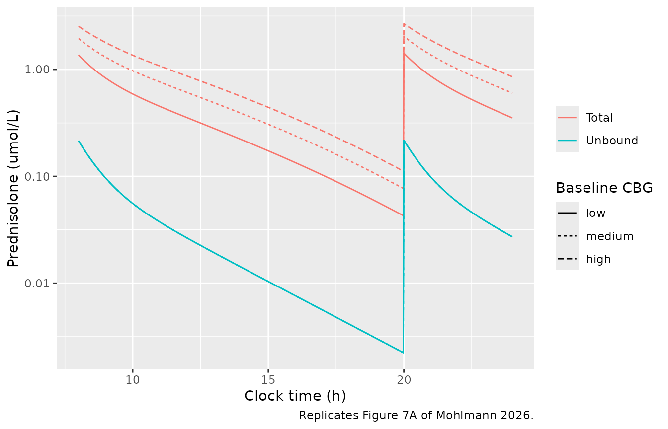
fig7a_sum <- fig7a |>
  dplyr::group_by(CBG) |>
  dplyr::summarise(
    cmax_tot = max(Ctot),
    fb_at_cmax = 1 - Cc[which.max(Ctot)] / Ctot[which.max(Ctot)],
    auc_tot = trap(time, Ctot),
    .groups = "drop"
  ) |>
  dplyr::mutate(fb_paper = c(0.84, 0.89, 0.92))
knitr::kable(
  fig7a_sum |>
    dplyr::mutate(dplyr::across(where(is.numeric), \(x) signif(x, 3))) |>
    dplyr::rename(
      "Baseline CBG" = CBG, "Cmax total (umol/L)" = cmax_tot,
      "Fraction bound at Cmax" = fb_at_cmax, "AUC0-24 total (umol*h/L)" = auc_tot,
      "Fraction bound, paper" = fb_paper
    ),
  caption = "Figure 7A typical patient; the paper reports the fraction bound at the maximum total concentration (Results 3.7)."
)| Baseline CBG | Cmax total (umol/L) | Fraction bound at Cmax | AUC0-24 total (umol*h/L) | Fraction bound, paper |
|---|---|---|---|---|
| low | 1.42 | 0.847 | 6.7 | 0.84 |
| medium | 2.05 | 0.894 | 10.9 | 0.89 |
| high | 2.68 | 0.919 | 15.1 | 0.92 |
ratio <- function(x) x / x[1]
fig7a_ratio <- data.frame(
  Comparison = c("Cmax total, medium vs low", "Cmax total, high vs low",
                 "AUC total, medium vs low", "AUC total, high vs low"),
  Simulated = round(c(ratio(fig7a_sum$cmax_tot)[2:3], ratio(fig7a_sum$auc_tot)[2:3]), 2),
  Paper = c(1.4, 1.9, 1.6, 2.3)
)
knitr::kable(fig7a_ratio, caption = "Fold-changes reported in Results 3.7.")| Comparison | Simulated | Paper |
|---|---|---|
| Cmax total, medium vs low | 1.44 | 1.4 |
| Cmax total, high vs low | 1.89 | 1.9 |
| AUC total, medium vs low | 1.62 | 1.6 |
| AUC total, high vs low | 2.26 | 2.3 |
# Deterministic typical-value predictions: tight bounds. A wrong KCBG, Kalb, Vc
# or unit conversion moves the fraction bound by several hundredths and the
# ratios by tenths.
stopifnot(
  all(abs(fig7a_sum$fb_at_cmax - fig7a_sum$fb_paper) < 0.015),
  all(abs(fig7a_ratio$Simulated - fig7a_ratio$Paper) < 0.1)
)
The paper also reports that the morning dose accounts for about 51% of the 24-h total AUC, a consequence of the circadian CBG rhythm. At steady state (fourth day of twice-daily dosing):
ss <- sim_typ(dose_times = seq(8, 8 + 24 * 4, by = 12), amt = 0.5 * 30 * 0.75, t_end = 24 * 5)
#> ℹ omega/sigma items treated as zero: 'etalvp', 'etalvc', 'etalcl', 'etalka'
morning_share <- auc_window(ss, "Ctot", 80, 92) / auc_window(ss, "Ctot", 80, 104)
cat(sprintf("Morning share of the 24-h total AUC: %.1f%% (paper: about 51%%)\n", 100 * morning_share))
#> Morning share of the 24-h total AUC: 50.2% (paper: about 51%)
# Unbound PK is linear and CBG-independent, so the unbound split is exactly
# 50:50 at steady state.
stopifnot(
  abs(morning_share - 0.51) < 0.02,
  abs(auc_window(ss, "Cc", 80, 92) / auc_window(ss, "Cc", 80, 104) - 0.5) < 0.002
)
Figure 7B: dosing regimen
regimens <- list(
  "0.5 mg/kg IV BID" = list(amt = 0.5 * 30 * 0.75, cmt = "central"),
  "0.5 mg/kg oral BID" = list(amt = 0.5 * 30, cmt = "depot"),
  "1 mg/kg oral BID" = list(amt = 1 * 30, cmt = "depot")
)
fig7b <- dplyr::bind_rows(lapply(names(regimens), function(nm) {
  r <- regimens[[nm]]
  sim_typ(dose_times = c(8, 20), amt = r$amt, cmt = r$cmt, t_end = 48) |>
    dplyr::mutate(regimen = nm)
}))
#> ℹ omega/sigma items treated as zero: 'etalvp', 'etalvc', 'etalcl', 'etalka'
#> ℹ omega/sigma items treated as zero: 'etalvp', 'etalvc', 'etalcl', 'etalka'
#> ℹ omega/sigma items treated as zero: 'etalvp', 'etalvc', 'etalcl', 'etalka'

fig7b |>
  dplyr::filter(time <= 24) |>
  tidyr::pivot_longer(c(Cc, Ctot), names_to = "analyte", values_to = "conc") |>
  dplyr::filter(conc > 0) |>
  dplyr::mutate(analyte = ifelse(analyte == "Cc", "Unbound", "Total")) |>
  ggplot(aes(time, conc, colour = analyte, linetype = regimen)) +
  geom_line() +
  scale_y_log10() +
  labs(x = "Clock time (h)", y = "Prednisolone (umol/L)", colour = NULL, linetype = NULL,
       caption = "Replicates Figure 7B of Mohlmann 2026.")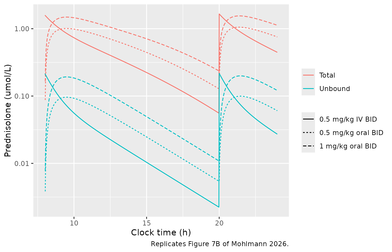
auc_reg <- fig7b |>
  dplyr::group_by(regimen) |>
  dplyr::summarise(auc_u = trap(time, Cc), auc_t = trap(time, Ctot),
                   tmax_after_dose = time[time <= 20][which.max(Ctot[time <= 20])] - 8,
                   .groups = "drop")
dbl_u <- auc_reg$auc_u[auc_reg$regimen == "1 mg/kg oral BID"] /
  auc_reg$auc_u[auc_reg$regimen == "0.5 mg/kg oral BID"]
dbl_t <- auc_reg$auc_t[auc_reg$regimen == "1 mg/kg oral BID"] /
  auc_reg$auc_t[auc_reg$regimen == "0.5 mg/kg oral BID"]
cat(sprintf("Doubling the oral dose: AUC unbound x %.2f (paper 2.0), AUC total x %.2f (paper 1.5)\n", dbl_u, dbl_t))
#> Doubling the oral dose: AUC unbound x 2.00 (paper 2.0), AUC total x 1.55 (paper 1.5)
cat(sprintf("Oral Tmax after the morning dose: %.1f h (paper: around 2 h)\n",
            auc_reg$tmax_after_dose[auc_reg$regimen == "0.5 mg/kg oral BID"]))
#> Oral Tmax after the morning dose: 1.5 h (paper: around 2 h)
stopifnot(
  # Unbound PK is linear, so the doubling is exact up to quadrature error.
  abs(dbl_u - 2) < 0.005,
  # Total is less than proportional because CBG saturates. The paper rounds
  # to one decimal, so anything in [1.45, 1.55] reads as 1.5.
  abs(dbl_t - 1.5) < 0.06
)
Figure 7C: clearance
Figure 7C varies CL in a 70 kg patient (62, 185 and 309 L/h). It is
simulated here by shifting etalcl, with 0.5 mg/kg IV twice
daily.
cl_levels <- c(low = 62, medium = 185, high = 309)
fig7c <- dplyr::bind_rows(lapply(names(cl_levels), function(nm) {
  sim_typ(dose_times = c(8, 20), amt = 0.5 * 70 * 0.75, wt = 70, t_end = 72,
          etalcl = log(cl_levels[[nm]] / 155)) |>
    dplyr::mutate(CL = nm)
}))
#> ℹ omega/sigma items treated as zero: 'etalvp', 'etalvc', 'etalcl', 'etalka'
#> ℹ omega/sigma items treated as zero: 'etalvp', 'etalvc', 'etalcl', 'etalka'
#> ℹ omega/sigma items treated as zero: 'etalvp', 'etalvc', 'etalcl', 'etalka'
fig7c$CL <- factor(fig7c$CL, levels = names(cl_levels))

fig7c |>
  dplyr::filter(time <= 24) |>
  tidyr::pivot_longer(c(Cc, Ctot), names_to = "analyte", values_to = "conc") |>
  dplyr::filter(conc > 0) |>
  dplyr::mutate(analyte = ifelse(analyte == "Cc", "Unbound", "Total")) |>
  ggplot(aes(time, conc, colour = analyte, linetype = CL)) +
  geom_line() +
  scale_y_log10() +
  labs(x = "Clock time (h)", y = "Prednisolone (umol/L)", colour = NULL, linetype = "CL",
       caption = "Replicates Figure 7C of Mohlmann 2026.")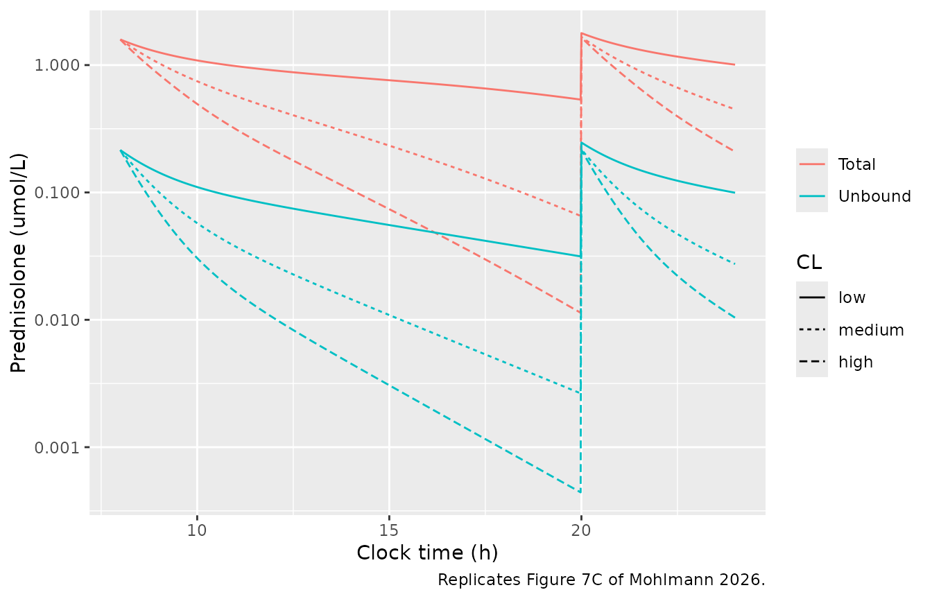
auc_cl <- fig7c |>
  dplyr::group_by(CL) |>
  dplyr::summarise(auc_u = trap(time, Cc), auc_t = trap(time, Ctot), .groups = "drop")
# Terminal half-life of the typical two-compartment system at each CL.
t_half_terminal <- sapply(cl_levels, function(cl) {
  kel <- cl / 338; k12 <- 105 / 338; k21 <- 105 / 170
  a <- kel + k12 + k21
  log(2) / ((a - sqrt(a^2 - 4 * kel * k21)) / 2)
})
knitr::kable(
  data.frame(
    CL = names(cl_levels),
    "AUC unbound, fold vs low" = round(auc_cl$auc_u[1] / auc_cl$auc_u, 2),
    "AUC total, fold vs low" = round(auc_cl$auc_t[1] / auc_cl$auc_t, 2),
    "Paper AUC total fold" = c(1, 2.8, 4.8),
    "Terminal t1/2 (h)" = round(unname(t_half_terminal), 1),
    "Paper t1/2 (h)" = c(4.9, 1.6, 1.0),
    check.names = FALSE,
    row.names = NULL
  ),
  caption = "Figure 7C: fold-decrease in AUC (0-72 h) relative to the low-CL patient, and half-lives."
)| CL | AUC unbound, fold vs low | AUC total, fold vs low | Paper AUC total fold | Terminal t1/2 (h) | Paper t1/2 (h) |
|---|---|---|---|---|---|
| low | 1.00 | 1.00 | 1.0 | 6.1 | 4.9 |
| medium | 2.97 | 2.74 | 2.8 | 2.4 | 1.6 |
| high | 4.94 | 4.57 | 4.8 | 1.8 | 1.0 |
The unbound AUC falls in proportion to CL. The simulated total AUC falls 2.7- and 4.6-fold where the paper prints 2.8- and 4.8-fold, and the printed half-lives (4.9, 1.6 and 1.0 h) are shorter than the terminal half-lives of the published parameters (6.1, 2.4, 1.8 h). The printed half-lives scale approximately as 1/CL with an implied volume of 430-450 L (half-life x CL / ln 2), which does not correspond to Vc (338 L) or Vc + Vp (508 L); the paper does not say how they were computed, so these two comparisons are reported rather than asserted.
Figure 7D: cohort
cohorts <- list(
  "Autoimmune (reference)" = c(tx_hct = 0, agvhd = 0),
  "HCT prophylaxis" = c(tx_hct = 1, agvhd = 0),
  "HCT therapy" = c(tx_hct = 1, agvhd = 1)
)
fig7d <- dplyr::bind_rows(lapply(names(cohorts), function(nm) {
  h <- cohorts[[nm]]
  sim_typ(dose_times = 8, amt = 1 * 30, cmt = "depot", t_end = 72,
          tx_hct = h[["tx_hct"]], agvhd = h[["agvhd"]]) |>
    dplyr::mutate(cohort = nm)
}))
#> ℹ omega/sigma items treated as zero: 'etalvp', 'etalvc', 'etalcl', 'etalka'
#> ℹ omega/sigma items treated as zero: 'etalvp', 'etalvc', 'etalcl', 'etalka'
#> ℹ omega/sigma items treated as zero: 'etalvp', 'etalvc', 'etalcl', 'etalka'
auc_coh <- fig7d |>
  dplyr::group_by(cohort) |>
  dplyr::summarise(auc_u = trap(time, Cc), auc_t = trap(time, Ctot), .groups = "drop")
ref <- auc_coh[auc_coh$cohort == "HCT prophylaxis", ]
others <- auc_coh[auc_coh$cohort != "HCT prophylaxis", ]
knitr::kable(
  data.frame(
    "Compared with" = others$cohort,
    "AUC unbound lower in HCT prophylaxis (%)" = round(100 * (1 - ref$auc_u / others$auc_u), 1),
    "AUC total lower in HCT prophylaxis (%)" = round(100 * (1 - ref$auc_t / others$auc_t), 1),
    check.names = FALSE
  ),
  caption = "Figure 7D, 1 mg/kg oral single dose. Paper (Results 3.7): 10.6-12.1% lower unbound and 9.1-10.3% lower total AUC."
)| Compared with | AUC unbound lower in HCT prophylaxis (%) | AUC total lower in HCT prophylaxis (%) |
|---|---|---|
| Autoimmune (reference) | 9.1 | 8.0 |
| HCT therapy | 11.4 | 10.1 |
# Linear unbound PK: the unbound difference is exactly 1 - 1/1.1 against the
# reference cohort.
stopifnot(abs(100 * (1 - ref$auc_u / others$auc_u[others$cohort == "Autoimmune (reference)"]) -
                100 * (1 - 1 / 1.1)) < 0.1)
The simulated differences (9.1-11.4% unbound, 8.0-10.1% total) sit up to about 1.5 percentage points below the paper’s ranges. Against the autoimmune cohort the unbound difference can only be 1 - 1/1.1 = 9.1% for linear unbound kinetics, so the paper’s lower bound of 10.6% is not reproducible from the published parameters; the source of the difference is not stated.
Virtual cohort
Two arms of 150 children each: an autoimmune arm (ages 6-18 years, a single oral 1 mg/kg dose at 8 AM) and an HCT arm (ages 0.5-18 years, a single IV 0.5 mg/kg dose of the succinate salt at 8 AM, half on prophylaxis and half on GvHD therapy). Weight is drawn around approximate 50th-percentile weight-for-age values with a 15% CV, albumin from a normal distribution matching Table 1, and baseline CBG log-normally around the observed median 1.04 umol/L, both kept inside the observed ranges by redrawing.
set.seed(20260101)
n_per_arm <- 150

# Approximate 50th-percentile weight-for-age (kg), both sexes.
wfa <- data.frame(
  age = c(0.5, 1, 2, 3, 4, 5, 6, 8, 10, 12, 14, 16, 18),
  wt = c(7.6, 9.6, 12.5, 14.3, 16.3, 18.4, 20.7, 25.8, 32.5, 40.5, 50, 58, 63)
)
# Reject-and-redraw keeps a draw inside its observed range without piling
# values up at the limits.
draw_in <- function(n, sampler, lo, hi) {
  out <- sampler(n)
  bad <- out < lo | out > hi
  while (any(bad)) {
    out[bad] <- sampler(sum(bad))
    bad <- out < lo | out > hi
  }
  out
}
draw_wt <- function(wt_med) {
  wt <- wt_med * exp(stats::rnorm(length(wt_med), 0, 0.15))
  bad <- wt < 5 | wt > 109
  while (any(bad)) {
    wt[bad] <- wt_med[bad] * exp(stats::rnorm(sum(bad), 0, 0.15))
    bad <- wt < 5 | wt > 109
  }
  wt
}
make_arm <- function(arm, age_lo) {
  age <- stats::runif(n_per_arm, age_lo, 18)
  data.frame(
    arm = arm,
    id = seq_len(n_per_arm),
    AGE = age,
    WT = draw_wt(stats::approx(wfa$age, wfa$wt, xout = age)$y),
    ALB = draw_in(n_per_arm, \(n) stats::rnorm(n, 31.1, 6), 13.9, 44.3),
    cbg_base = draw_in(n_per_arm, \(n) stats::rlnorm(n, log(1.04), 0.3), 0.60, 2.48)
  )
}
subjects <- dplyr::bind_rows(make_arm("Autoimmune, oral", 6), make_arm("HCT, IV", 0.5)) |>
  dplyr::mutate(
    TX_HCT = as.integer(arm == "HCT, IV"),
    AGVHD_ANY = as.integer(arm == "HCT, IV" & id > n_per_arm / 2),
    amt = ifelse(arm == "HCT, IV", 0.5 * WT * 0.75, 1 * WT),
    cmt = ifelse(arm == "HCT, IV", "central", "depot")
  )
stopifnot(abs(stats::median(subjects$ALB) - 31.1) < 2,
          abs(stats::median(subjects$cbg_base) - 1.04) < 0.1)
grid <- sort(unique(c(seq(0, 2, by = 0.05), seq(2, 8, by = 0.1), seq(8, 48, by = 0.25))))
cohort_events <- dplyr::bind_rows(lapply(seq_len(nrow(subjects)), function(i) {
  s <- subjects[i, ]
  ev <- rbind(
    data.frame(time = 0, amt = s$amt, cmt = s$cmt, evid = 1L, dvid = NA_integer_),
    data.frame(time = grid, amt = NA_real_, cmt = "central", evid = 0L, dvid = 1L)
  )
  ev <- ev[order(ev$time, -ev$evid), ]
  ev$id <- s$id; ev$arm <- s$arm
  ev$WT <- s$WT; ev$ALB <- s$ALB; ev$TX_HCT <- s$TX_HCT; ev$AGVHD_ANY <- s$AGVHD_ANY
  # Dose at 8 AM: time 0 is clock 8 h.
  ev$TRANSCORTIN <- cbg_curve_um(ev$time + 8, s$cbg_base) * mw_cbg_kda
  ev
}))
Simulated profiles (compare Figure 6)
# Each arm is solved separately because the IDs are reused across arms.
sim_vpc <- dplyr::bind_rows(lapply(unique(subjects$arm), function(a) {
  rxode2::rxSolve(mod, dplyr::filter(cohort_events, arm == a),
                  keep = c("arm"), returnType = "data.frame") |>
    as.data.frame()
}))
sim_vpc |>
  dplyr::filter(time > 0, time <= 12) |>
  tidyr::pivot_longer(c(Cc, Ctot), names_to = "analyte", values_to = "conc") |>
  dplyr::mutate(analyte = ifelse(analyte == "Cc", "Unbound", "Total")) |>
  dplyr::group_by(arm, analyte, time) |>
  dplyr::summarise(p10 = stats::quantile(conc, 0.1), p50 = stats::median(conc),
                   p90 = stats::quantile(conc, 0.9), .groups = "drop") |>
  ggplot(aes(time, p50, colour = analyte, fill = analyte)) +
  geom_ribbon(aes(ymin = p10, ymax = p90), alpha = 0.2, colour = NA) +
  geom_line() +
  facet_wrap(~arm) +
  scale_y_log10() +
  labs(x = "Time after dose (h)", y = "Prednisolone (umol/L)", colour = NULL, fill = NULL,
       caption = "Median and 10th-90th percentiles of the simulated individual profiles, without residual error. Compare Figure 6 of Mohlmann 2026.")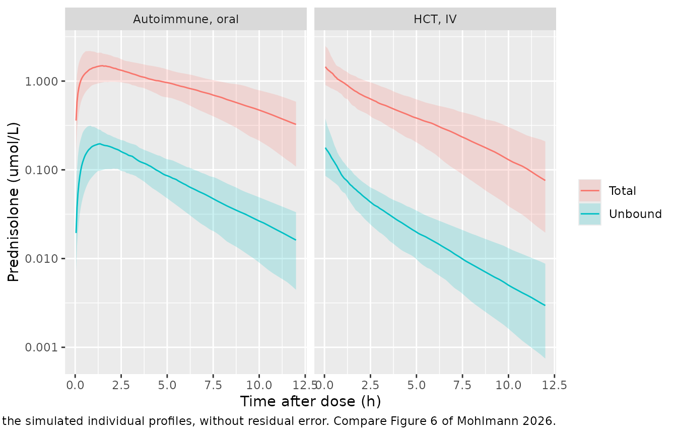
PKNCA validation
The paper reports no NCA table, so PKNCA is used to summarise the simulated exposure and to check the model’s mass balance: because elimination is linear in unbound prednisolone and the dose enters the unbound pool with F = 1, each subject’s CL times unbound AUC to infinity (converted to mg*h/L by dividing by 2.77) must return the administered dose.
# Between-subject variability on, residual error off: the mass-balance
# identity is a property of the ODE system, and residual noise would only blur
# AUC.
mod_nores <- rxode2::zeroRe(mod, which = "sigma")
sim_nca_raw <- dplyr::bind_rows(lapply(unique(subjects$arm), function(a) {
  rxode2::rxSolve(mod_nores, dplyr::filter(cohort_events, arm == a),
                  keep = c("arm"), returnType = "data.frame") |>
    as.data.frame()
}))
stopifnot(all(sim_nca_raw$Cc >= 0), all(sim_nca_raw$Ctot >= sim_nca_raw$Cc))
run_nca <- function(conc_col) {
  conc <- sim_nca_raw |>
    dplyr::filter(!is.na(.data[[conc_col]])) |>
    dplyr::select(id, time, arm, conc = dplyr::all_of(conc_col))
  # Guarantee a time = 0 record per subject; pre-dose prednisolone is 0.
  conc <- dplyr::bind_rows(conc, conc |> dplyr::distinct(id, arm) |> dplyr::mutate(time = 0, conc = 0)) |>
    dplyr::distinct(id, arm, time, .keep_all = TRUE) |>
    dplyr::arrange(arm, id, time)
  conc_obj <- PKNCA::PKNCAconc(conc, conc ~ time | arm + id, concu = "umol/L", timeu = "h")
  dose_obj <- PKNCA::PKNCAdose(
    subjects |> dplyr::mutate(time = 0) |> dplyr::select(id, arm, time, amt),
    amt ~ time | arm + id, doseu = "mg"
  )
  intervals <- data.frame(start = 0, end = Inf, cmax = TRUE, tmax = TRUE,
                          aucinf.obs = TRUE, half.life = TRUE)
  PKNCA::pk.nca(PKNCA::PKNCAdata(conc_obj, dose_obj, intervals = intervals)) |>
    as.data.frame() |>
    dplyr::select(arm, id, PPTESTCD, PPORRES) |>
    tidyr::pivot_wider(names_from = PPTESTCD, values_from = PPORRES)
}
nca_u <- run_nca("Cc")
nca_t <- run_nca("Ctot")
stopifnot(nrow(nca_u) == 2 * n_per_arm, !anyNA(nca_u$aucinf.obs), !anyNA(nca_t$aucinf.obs))

nca_tab <- dplyr::bind_rows(
  nca_u |> dplyr::mutate(analyte = "Unbound"),
  nca_t |> dplyr::mutate(analyte = "Total")
) |>
  dplyr::group_by(arm, analyte) |>
  dplyr::summarise(
    cmax = sprintf("%.3g (%.3g-%.3g)", stats::median(cmax), stats::quantile(cmax, 0.05), stats::quantile(cmax, 0.95)),
    tmax = sprintf("%.2g", stats::median(tmax)),
    auc = sprintf("%.3g (%.3g-%.3g)", stats::median(aucinf.obs), stats::quantile(aucinf.obs, 0.05), stats::quantile(aucinf.obs, 0.95)),
    thalf = sprintf("%.2g", stats::median(half.life)),
    .groups = "drop"
  ) |>
  dplyr::rename("Arm" = arm, "Analyte" = analyte, "Cmax (umol/L)" = cmax,
                "Tmax (h)" = tmax, "AUC0-inf (umol*h/L)" = auc, "t1/2 (h)" = thalf)
knitr::kable(nca_tab, caption = "Single-dose NCA, median (5th-95th percentile). Autoimmune: 1 mg/kg oral; HCT: 0.5 mg/kg IV succinate (0.375 mg/kg prednisolone).")| Arm | Analyte | Cmax (umol/L) | Tmax (h) | AUC0-inf (umol*h/L) | t1/2 (h) |
|---|---|---|---|---|---|
| Autoimmune, oral | Total | 1.45 (0.885-2.37) | 1.5 | 11.9 (6.69-20.1) | 2.7 |
| Autoimmune, oral | Unbound | 0.177 (0.0957-0.356) | 1.5 | 1.04 (0.607-1.65) | 2.6 |
| HCT, IV | Total | 1.67 (1-3.08) | 0 | 5.13 (2.75-10.1) | 2.5 |
| HCT, IV | Unbound | 0.226 (0.0815-0.597) | 0 | 0.371 (0.195-0.657) | 2.4 |
cl_per_id <- sim_nca_raw |>
  dplyr::group_by(arm, id) |>
  dplyr::summarise(cl = dplyr::first(cl), .groups = "drop")
mb <- nca_u |>
  dplyr::left_join(cl_per_id, by = c("arm", "id")) |>
  dplyr::left_join(subjects |> dplyr::select(arm, id, amt), by = c("arm", "id")) |>
  dplyr::mutate(pct_diff = 100 * (cl * aucinf.obs / 2.77 - amt) / amt)
knitr::kable(
  mb |>
    dplyr::group_by(arm) |>
    dplyr::summarise(median = round(stats::median(pct_diff), 3),
                     max_abs = round(max(abs(pct_diff)), 3), .groups = "drop") |>
    dplyr::rename("Arm" = arm, "Median CL*AUC/dose - 1 (%)" = median, "Max |diff| (%)" = max_abs),
  caption = "Mass balance on unbound prednisolone."
)| Arm | Median CL*AUC/dose - 1 (%) | Max |diff| (%) |
|---|---|---|
| Autoimmune, oral | -0.010 | 0.056 |
| HCT, IV | 0.005 | 0.023 |
Assumptions and deviations
- Dose clock times. The paper does not state when the Figure 7 doses were given; 8 AM and 8 PM are assumed. Only the circadian CBG term depends on this, and the 51% morning-AUC share is reproduced under that assumption.
-
CBG is a supplied covariate, not computed in the
model. Following the control stream, the model reads a
time-varying CBG column (
TRANSCORTIN, mg/L). The vignette rebuilds it with Eqs 7-8 from a baseline value. In the study the baseline itself was an empirical Bayes estimate from one measurement per occasion with the Melin et al. model. -
IV doses are the salt-corrected amount. The data
column
AMTis the prednisolone amount after correcting the sodium succinate salt by 0.75; dose IV prednisolone as0.75 xthe labelled salt dose intocentral. Results 3.7 states the 0.75 conversion factor, and the Figure 7A fraction-bound values are reproduced with it. -
AUC bookkeeping states omitted. The control stream
integrates unbound and total AUC in two extra compartments
(
AUCU,AUCT) for its table output; they do not affect the PK and are not included. Compute AUC fromCcandCtot. -
The cohort covariate is encoded with
TX_HCTandAGVHD_ANY; the paper’s HCT-therapy level also includes engraftment syndrome treated with the same 2 mg/kg/day regimen. - Unreproduced numbers. The Figure 7C half-lives and the lower end of the Figure 7D AUC differences do not follow from the published parameters (see above). They are reported, not asserted.
- Virtual cohort. Weight-for-age medians, albumin and CBG distributions are approximations matched to the Table 1 centre and range; the paper’s individual covariates are not available.
- Screened covariates not in the model. Sex, age, maturation (postmenstrual age), CYP3A4 inhibitors, cyclosporin A, antithymocyte globulin, liver function and oral formulation were tested and not retained (Results 3.4); IOV and an estimated F (1.17) were also rejected (Results 3.3).