Tenofovir from TDF or TAF (Kawuma 2023)
Source:vignettes/articles/Kawuma_2023_tenofovir.Rmd
Kawuma_2023_tenofovir.RmdModel and source
- Citation: Kawuma AN, Wasmann RE, Sinxadi P, Sokhela SM, Chandiwana N, Venter WDF, Wiesner L, Maartens G, Denti P. Population pharmacokinetics of tenofovir given as either tenofovir disoproxil fumarate or tenofovir alafenamide in an African population. CPT Pharmacometrics Syst Pharmacol. 2023;12(6):821-830. doi:10.1002/psp4.12955
- Description: Joint semimechanistic two-compartment population PK model for plasma tenofovir when administered as either tenofovir disoproxil fumarate (TDF) or tenofovir alafenamide (TAF) in South African adults living with HIV (Kawuma 2023). Both prodrugs share one tenofovir disposition model; TDF appears in plasma by a single first-order process, whereas a TAF dose splits into a fast fraction absorbed first-order into the systemic circulation and a slow fraction sequestered in an intracellular reservoir (interpreted as PBMCs) that releases tenofovir with a fixed 6.83-day half-life. Doses are expressed as tenofovir-equivalent amounts.
- Article: https://doi.org/10.1002/psp4.12955
Tenofovir disoproxil fumarate (TDF) and tenofovir alafenamide (TAF) are both prodrugs of tenofovir. TDF converts to tenofovir largely in plasma, whereas TAF is taken up into cells and converted there, so TAF can be given at a much lower dose and produces roughly ten-fold lower plasma tenofovir concentrations.
Kawuma 2023 is notable for fitting one tenofovir disposition model to both prodrugs. The authors argue explicitly against the earlier approach of Greene et al., who fitted TDF and TAF separately and reported two clearance values differing about ten-fold: once tenofovir has reached plasma it should be distributed and eliminated the same way regardless of which prodrug delivered it. In this model the ten-fold exposure difference is produced entirely by the input function, not by the disposition.
Consequently the model has three input compartments and one shared two- compartment disposition:
| Compartment | Fed by | Rate out |
|---|---|---|
depot |
a TDF dose |
Ka_TDF = 3.04 /h |
depot2 |
the fast fraction of a TAF dose |
Ka_TAF = 1.45 /h |
depot3 |
the slow fraction of a TAF dose, sequestered intracellularly | half-life 6.83 days |
Doses are tenofovir-equivalent amounts
The model’s dosing unit is mg of tenofovir, not mg of prodrug. Kawuma 2023 Methods converts by molecular weight (tenofovir 287.2 g/mol; TDF 635.5 g/mol; TAF 476.5 g/mol):
mw_tfv <- 287.2
mw_tdf <- 635.5
mw_taf <- 476.5

# The paper's own rounded conversions (Methods): 300 mg TDF -> 136 mg
# tenofovir; 25 mg TAF -> 15 mg tenofovir.
tfv_tdf300 <- 136
tfv_taf25 <- 15
# 10 mg TAF is simulated in Table 3 but its conversion is not printed.
tfv_taf10 <- 10 * mw_tfv / mw_taf

c(
  check_tdf300 = 300 * mw_tfv / mw_tdf,
  check_taf25 = 25 * mw_tfv / mw_taf,
  taf10 = tfv_taf10
)
#> check_tdf300  check_taf25        taf10
#>   135.578285    15.068206     6.027282
135.6 and 15.07 round to the paper’s 136 mg and 15 mg, confirming the conversion.
Population
The model was built on 279 tenofovir concentrations from 41 South African adults living with HIV, enrolled in a pharmacokinetic substudy nested within the ADVANCE trial (NCT03122262). Twenty-one participants received TDF 300 mg and twenty received TAF 25 mg, each co-formulated with emtricitabine 200 mg and given with dolutegravir 50 mg once daily. Sampling was rich – predose and at 1, 2, 4, 6, 8 and 24 h postdose – and was performed after at least 48 weeks of treatment, so every profile is at steady state.
Baseline characteristics (Kawuma 2023 Table 1, “ALL” column): median (IQR) age 31.0 (29.0-36.0) years, weight 73.1 (67.2-85.2) kg, height 167 (161-174) cm, and Cockcroft-Gault creatinine clearance at screening 120 (96.0-140) mL/min. 27 of 41 participants (65.9%) were female. None of the 279 samples fell below the 0.0005 mg/L limit of quantification.
The same information is available programmatically:
str(rxode2::rxode2(readModelDb("Kawuma_2023_tenofovir"))$population)
#> ℹ parameter labels from comments will be replaced by 'label()'
#> Warning: some etas defaulted to non-mu referenced, possible parsing error: etaiov_fdepot_tdf_1, etaiov_fdepot_tdf_2, etaiov_ka_tdf_1, etaiov_ka_tdf_2, etaiov_ka_taf_1, etaiov_ka_taf_2
#> as a work-around try putting the mu-referenced expression on a simple line
#> List of 15
#>  $ species       : chr "human"
#>  $ n_subjects    : num 41
#>  $ n_studies     : num 1
#>  $ n_observations: num 279
#>  $ age_median    : chr "31.0 years (IQR 29.0-36.0)"
#>  $ weight_median : chr "73.1 kg (IQR 67.2-85.2)"
#>  $ height_median : chr "167 cm (IQR 161-174)"
#>  $ sex_female_pct: num 65.9
#>  $ race_ethnicity: chr "South African adults; the source paper reports no race or ethnicity breakdown."
#>  $ renal_function: chr "Creatinine clearance at screening (Cockcroft-Gault) median 120 mL/min (IQR 96.0-140); no participant had impair"| __truncated__
#>  $ disease_state : chr "Treatment-naive adults living with HIV, sampled after at least 48 weeks of antiretroviral therapy."
#>  $ dose_range    : chr "TDF 300 mg once daily (= 136 mg tenofovir) in 21 participants, or TAF 25 mg once daily (= 15 mg tenofovir) in 2"| __truncated__
#>  $ co_medication : chr "Dolutegravir 50 mg and emtricitabine 200 mg once daily in both arms."
#>  $ regions       : chr "South Africa"
#>  $ notes         : chr "Pharmacokinetic substudy nested within the ADVANCE trial (NCT03122262), an open-label phase III randomized noni"| __truncated__
Source trace
Every value in ini() and every non-obvious equation in
model(), with the place in Kawuma 2023 it came from.
| Model element | Value | Source |
|---|---|---|
lcl |
CL 44.7 L/h (40.2-49.5) | Table 2, CL (L/h) row |
lvc |
Vc 378 L (319-459) | Table 2, Vc (L) row |
lq |
Q 157 L/h (103-233) | Table 2, Q (L/h) row |
lvp |
Vp 356 L (298-438) | Table 2, Vp (L) row |
e_wt_cl_q |
0.75, fixed | Methods: “allometric exponents for clearance and volume were fixed to 0.75 and 1” |
e_wt_vc_vp |
1, fixed | Methods, as above |
| reference weight | 70 kg | Table 2 footnote c; Results “For a typical individual of 70 kg” |
lka_tdf |
Ka_TDF 3.04 /h (2.11-3.88) | Table 2, Ka_TDF (1/h) row |
lfdepot_tdf |
F_TDF 1, fixed | Table 2, F_TDF row, “1-Fixed” |
lfdepot_taf |
F_TAF 0.822 (0.723-0.939) | Table 2, F_TAF row; Results text repeats 82.2%
(72.3-93.9) |
logitffo |
Frac_TAF-Fast 32.4% (27.0-37.7) | Table 2, Frac_TAF-Fast (%) row |
lka_taf_fast |
Ka_TAF 1.45 /h (0.924-2.60) | Table 2, Ka_TAF (1/h) row |
lka_taf_slow |
t1/2 6.83 days, fixed; rate = log(2)/(6.83 x 24) /h | Table 2, t1/2_TAF-Slow, days row, “6.83-Fixed” |
etalcl |
BSV on CL 20.1% (16.1-24.7) | Table 2 CL row, variability column, footnote d |
etaiov_fdepot_tdf_* |
BOV on F_TDF 23.9% (18.2-30.3) | Table 2 F_TDF row, footnote e |
etaiov_ka_tdf_* |
BOV on Ka_TDF 114.5% (68.4-162) | Table 2 Ka_TDF row, footnote e |
etaiov_ka_taf_* |
BOV on Ka_TAF 66.3% (31.0-91.6) | Table 2 Ka_TAF row, footnote e |
| variance scale | omega^2 = (CV%/100)^2 | Table 2 footnote b: “calculated by CV% = sqrt(omega^2) x 100” |
propSd |
11.9% (10.8-13.4) | Table 2, Proportional error (%) row |
addSd |
0.2 x 0.0005 = 0.0001 mg/L, fixed | Table 2 Additive error row “20% of LLOQ-Fixed”;
footnote f “The LLOQ was 0.0005 mg/L” |
| two parallel TAF pathways | structure | Figure 2 legend; Results paragraph 3 |
| two-compartment disposition | structure | Results: “A two-compartment disposition model (dOFV = -47…) best described” |
| occasion definition | 2 occasions | Methods: “an ‘occasion’ was defined as a dose with its proceeding sample” |
| dose conversion | 136 mg / 15 mg tenofovir | Methods, “Population pharmacokinetic modeling” paragraph 1 |
Note the variance scale. Table 2 footnote b defines
CV% = sqrt(omega^2) * 100, i.e. the printed percentages are
omega on the standard-deviation scale directly. The variances in
ini() are therefore (CV/100)^2 and
not the exp-based log(1 + CV^2) conversion
that many popPK papers imply.
How a dose is given to this model
A TDF regimen doses depot only. A
TAF regimen doses both
depot2 and depot3 with the same
tenofovir-equivalent amount; the f() terms in the model
split that amount between the fast and slow pathways so that the two
records together deliver F_TAF worth of one dose:
f(depot2) = F_TAF * Frac_TAF-Fast
f(depot3) = F_TAF * (1 - Frac_TAF-Fast)
mod <- rxode2::rxode2(readModelDb("Kawuma_2023_tenofovir"))
#> ℹ parameter labels from comments will be replaced by 'label()'
#> Warning: some etas defaulted to non-mu referenced, possible parsing error: etaiov_fdepot_tdf_1, etaiov_fdepot_tdf_2, etaiov_ka_tdf_1, etaiov_ka_tdf_2, etaiov_ka_taf_1, etaiov_ka_taf_2
#> as a work-around try putting the mu-referenced expression on a simple line

#' Build an event table for one arm.
#'
#' @param tfv_dose tenofovir-equivalent dose in mg
#' @param arm "TDF" or "TAF"
#' @param ndays number of once-daily doses
#' @param obs_from,obs_to,obs_by observation grid, in hours
build_events <- function(tfv_dose, arm, ndays, obs_from, obs_to, obs_by) {
  last_dose <- 24 * (ndays - 1)
  ev <-
    if (arm == "TDF") {
      rxode2::et(amt = tfv_dose, cmt = "depot", ii = 24, until = last_dose)
    } else {
      rxode2::et(amt = tfv_dose, cmt = "depot2", ii = 24, until = last_dose) |>
        rxode2::et(amt = tfv_dose, cmt = "depot3", ii = 24, until = last_dose)
    }
  # Observe on the ODE state `central`; rxode2 returns the algebraic
  # observable Cc as a column at those records.
  rxode2::et(ev, seq(obs_from, obs_to, by = obs_by), cmt = "central")
}
Both arms are solved with OCC = 0, which zeroes every
occasion indicator and so removes the between-occasion contribution.
This matches how the authors ran their own simulations (Table 3 footnote
a: “excluding between-occasion variability on absorption
parameters”).
Structure check: where the tenofovir comes from
A single 25 mg TAF dose, split into the two pathways, shows the
mechanism the paper describes: a fast peak within the first few hours
from depot2, then a long, almost flat tail sustained by
slow release from the intracellular reservoir depot3.
ev_single <- build_events(tfv_taf25, "TAF", ndays = 1,
                          obs_from = 0, obs_to = 24 * 21, obs_by = 0.5)
#> Warning: 'time'+'ii' is greater than 'until', no additional doses added
#> Warning: 'ii' requires non zero additional doses ('addl') or steady state
#> dosing ('ii': 24.000000, 'ss': 0; 'addl': 0), reset 'ii' to zero
#> Warning: 'time'+'ii' is greater than 'until', no additional doses added
#> Warning: 'ii' requires non zero additional doses ('addl') or steady state
#> dosing ('ii': 24.000000, 'ss': 0; 'addl': 0), reset 'ii' to zero
d_single <- as.data.frame(ev_single)
d_single$WT <- 70
d_single$OCC <- 0

sim_single <-
  rxode2::rxSolve(rxode2::zeroRe(mod), d_single, returnType = "data.frame")
#> Warning: some etas defaulted to non-mu referenced, possible parsing error: etaiov_fdepot_tdf_1, etaiov_fdepot_tdf_2, etaiov_ka_tdf_1, etaiov_ka_tdf_2, etaiov_ka_taf_1, etaiov_ka_taf_2
#> as a work-around try putting the mu-referenced expression on a simple line
#> ℹ omega/sigma items treated as zero: 'etalcl', 'etaiov_fdepot_tdf_1', 'etaiov_fdepot_tdf_2', 'etaiov_ka_tdf_1', 'etaiov_ka_tdf_2', 'etaiov_ka_taf_1', 'etaiov_ka_taf_2'

sim_single |>
  filter(!is.na(Cc)) |>
  select(time, depot2, depot3) |>
  pivot_longer(c(depot2, depot3), names_to = "compartment",
               values_to = "amount_mg") |>
  mutate(compartment = recode(compartment,
                              depot2 = "depot2 (fast pathway)",
                              depot3 = "depot3 (intracellular reservoir)")) |>
  ggplot(aes(time / 24, amount_mg, colour = compartment)) +
  geom_line(linewidth = 0.8) +
  labs(x = "Days since dose", y = "Tenofovir remaining (mg)",
       colour = NULL) +
  theme_bw() +
  theme(legend.position = "top")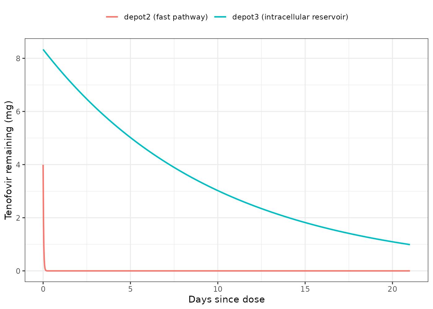
Single-dose tenofovir after TAF 25 mg, typical 70 kg individual, showing the amount remaining in each TAF input compartment. Replicates the mechanism drawn in Figure 2 of Kawuma 2023.
The fast pathway is essentially exhausted within a day while the reservoir is still nearly full, which is what produces tenofovir’s much longer apparent plasma half-life after TAF than after TDF. Ruane et al. (cited in the Kawuma 2023 Discussion) measured 14.86 h after TDF versus 40.19 h after TAF; here that difference is generated by the input function while disposition is held identical.
# Fraction of the administered tenofovir amount routed down each pathway.
# The model applies f() at the dose record, so the amount in each depot at
# t = 0+ is the check.
t0 <- sim_single |> filter(!is.na(Cc)) |> slice_min(time, n = 1)
c(
  fast_mg = t0$depot2,
  slow_mg = t0$depot3,
  total_mg = t0$depot2 + t0$depot3,
  expected_total_mg = tfv_taf25 * 0.822,
  fast_fraction = t0$depot2 / (t0$depot2 + t0$depot3)
)
#>           fast_mg           slow_mg          total_mg expected_total_mg
#>           3.99492           8.33508          12.33000          12.33000
#>     fast_fraction
#>           0.32400

stopifnot(
  # The two records together deliver exactly F_TAF of the dose ...
  abs((t0$depot2 + t0$depot3) - tfv_taf25 * 0.822) < 1e-6,
  # ... split in the published 32.4 / 67.6 ratio.
  abs(t0$depot2 / (t0$depot2 + t0$depot3) - 0.324) < 1e-6
)
Steady state takes weeks on TAF, days on TDF
The reservoir’s 6.83-day half-life means a TAF regimen needs roughly five of those half-lives – about 34 days – before the slow pathway stops accumulating. TDF, with no reservoir, reaches steady state within a few days. We therefore run 45 once-daily doses and take the final dosing interval for both arms, so the same run-in covers the slower arm.
n_days_ss <- 45

approach <- bind_rows(
  lapply(
    list(
      list(arm = "TDF", dose = tfv_tdf300),
      list(arm = "TAF", dose = tfv_taf25)
    ),
    function(a) {
      d <- as.data.frame(
        build_events(a$dose, a$arm, ndays = n_days_ss,
                     obs_from = 0, obs_to = 24 * n_days_ss, obs_by = 3)
      )
      d$WT <- 70
      d$OCC <- 0
      out <- rxode2::rxSolve(rxode2::zeroRe(mod), d, returnType = "data.frame")
      out$arm <- a$arm
      out[!is.na(out$Cc), c("time", "Cc", "arm")]
    }
  )
)
#> Warning: some etas defaulted to non-mu referenced, possible parsing error: etaiov_fdepot_tdf_1, etaiov_fdepot_tdf_2, etaiov_ka_tdf_1, etaiov_ka_tdf_2, etaiov_ka_taf_1, etaiov_ka_taf_2
#> as a work-around try putting the mu-referenced expression on a simple line
#> ℹ omega/sigma items treated as zero: 'etalcl', 'etaiov_fdepot_tdf_1', 'etaiov_fdepot_tdf_2', 'etaiov_ka_tdf_1', 'etaiov_ka_tdf_2', 'etaiov_ka_taf_1', 'etaiov_ka_taf_2'
#> Warning: some etas defaulted to non-mu referenced, possible parsing error: etaiov_fdepot_tdf_1, etaiov_fdepot_tdf_2, etaiov_ka_tdf_1, etaiov_ka_tdf_2, etaiov_ka_taf_1, etaiov_ka_taf_2
#> as a work-around try putting the mu-referenced expression on a simple line
#> ℹ omega/sigma items treated as zero: 'etalcl', 'etaiov_fdepot_tdf_1', 'etaiov_fdepot_tdf_2', 'etaiov_ka_tdf_1', 'etaiov_ka_tdf_2', 'etaiov_ka_taf_1', 'etaiov_ka_taf_2'

ggplot(approach, aes(time / 24, Cc * 1000)) +
  geom_line(linewidth = 0.7) +
  facet_wrap(~arm, scales = "free_y") +
  labs(x = "Days", y = "Plasma tenofovir (ng/mL)") +
  theme_bw()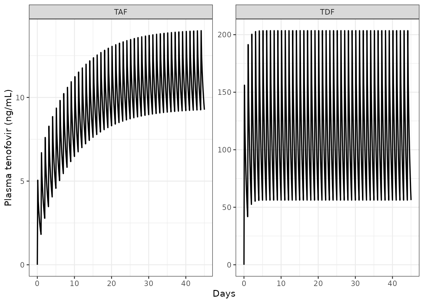
Approach to steady state on once-daily dosing, typical 70 kg individual. Tenofovir from TAF accumulates over about a month because of the intracellular reservoir; tenofovir from TDF plateaus within days.
# Trough on the last day vs the day before: both arms must have plateaued.
trough_ratio <- approach |>
  filter(time %in% c(24 * (n_days_ss - 1), 24 * (n_days_ss - 2))) |>
  group_by(arm) |>
  summarise(ratio = Cc[time == max(time)] / Cc[time == min(time)],
            .groups = "drop")
trough_ratio
#> # A tibble: 2 × 2
#>   arm   ratio
#>   <chr> <dbl>
#> 1 TAF    1.00
#> 2 TDF    1.00

stopifnot(all(abs(trough_ratio$ratio - 1) < 0.01))
Replicating the published simulated AUC (Table 3)
Kawuma 2023 Table 3 compares AUC0-24h simulated with the final model
against values reported by three other studies. The simulated column is
the model prediction we can check directly. The authors state their AUCs
were obtained as AUC0-24h = F_i * Dose_i / CL_i for “1000
runs of a single typical individual of the weight and dose specified per
study excluding between-occasion variability on absorption parameters”,
so the target is a typical-value prediction. We therefore simulate with
zeroRe() and compute the AUC over the final dosing interval
by NCA – an independent route to the same number, which also exercises
the ODE mass balance, the f() splits and the allometry.
scenarios <- tibble::tribble(
  ~scenario,                ~arm,  ~wt,  ~tfv_dose,   ~auclast_ref,
  "TDF 300 mg, 77 kg",      "TDF", 77.0, tfv_tdf300,  2795,
  "TDF 300 mg, 52 kg",      "TDF", 52.0, tfv_tdf300,  3761,
  "TAF 25 mg, 77 kg",       "TAF", 77.0, tfv_taf25,   253.6,
  "TAF 25 mg, 78.7 kg",     "TAF", 78.7, tfv_taf25,   259.8,
  "TAF 10 mg, 77 kg",       "TAF", 77.0, tfv_taf10,   101.6,
  "TAF 10 mg, 74.3 kg",     "TAF", 74.3, tfv_taf10,   108.6
)
knitr::kable(
  scenarios |> select(-arm) |> rename("Scenario" = scenario,
                                      "Weight (kg)" = wt,
                                      "Tenofovir dose (mg)" = tfv_dose,
                                      "Published AUC0-24 (ng*h/mL)" = auclast_ref),
  digits = 2,
  caption = "Simulation scenarios and the corresponding published model-simulated AUC0-24h, from Kawuma 2023 Table 3."
)| Scenario | Weight (kg) | Tenofovir dose (mg) | Published AUC0-24 (ng*h/mL) |
|---|---|---|---|
| TDF 300 mg, 77 kg | 77.0 | 136.00 | 2795.0 |
| TDF 300 mg, 52 kg | 52.0 | 136.00 | 3761.0 |
| TAF 25 mg, 77 kg | 77.0 | 15.00 | 253.6 |
| TAF 25 mg, 78.7 kg | 78.7 | 15.00 | 259.8 |
| TAF 10 mg, 77 kg | 77.0 | 6.03 | 101.6 |
| TAF 10 mg, 74.3 kg | 74.3 | 6.03 | 108.6 |
start_ss <- 24 * (n_days_ss - 1)
end_ss <- 24 * n_days_ss

# One rxSolve call per scenario; solving an rxUi scales poorly when many
# subjects go through a single call.
ss_conc <- bind_rows(lapply(seq_len(nrow(scenarios)), function(i) {
  s <- scenarios[i, ]
  d <- as.data.frame(
    build_events(s$tfv_dose, s$arm, ndays = n_days_ss,
                 obs_from = start_ss, obs_to = end_ss, obs_by = 0.1)
  )
  d$WT <- s$wt
  d$OCC <- 0
  out <- rxode2::rxSolve(rxode2::zeroRe(mod), d, returnType = "data.frame")
  out <- out[!is.na(out$Cc), ]
  data.frame(
    scenario = s$scenario,
    id = 1L,
    time = out$time,
    # mg/L -> ng/mL so the NCA output is directly in the paper's units
    conc = out$Cc * 1000
  )
}))
#> Warning: some etas defaulted to non-mu referenced, possible parsing error: etaiov_fdepot_tdf_1, etaiov_fdepot_tdf_2, etaiov_ka_tdf_1, etaiov_ka_tdf_2, etaiov_ka_taf_1, etaiov_ka_taf_2
#> as a work-around try putting the mu-referenced expression on a simple line
#> ℹ omega/sigma items treated as zero: 'etalcl', 'etaiov_fdepot_tdf_1', 'etaiov_fdepot_tdf_2', 'etaiov_ka_tdf_1', 'etaiov_ka_tdf_2', 'etaiov_ka_taf_1', 'etaiov_ka_taf_2'
#> Warning: some etas defaulted to non-mu referenced, possible parsing error: etaiov_fdepot_tdf_1, etaiov_fdepot_tdf_2, etaiov_ka_tdf_1, etaiov_ka_tdf_2, etaiov_ka_taf_1, etaiov_ka_taf_2
#> as a work-around try putting the mu-referenced expression on a simple line
#> ℹ omega/sigma items treated as zero: 'etalcl', 'etaiov_fdepot_tdf_1', 'etaiov_fdepot_tdf_2', 'etaiov_ka_tdf_1', 'etaiov_ka_tdf_2', 'etaiov_ka_taf_1', 'etaiov_ka_taf_2'
#> Warning: some etas defaulted to non-mu referenced, possible parsing error: etaiov_fdepot_tdf_1, etaiov_fdepot_tdf_2, etaiov_ka_tdf_1, etaiov_ka_tdf_2, etaiov_ka_taf_1, etaiov_ka_taf_2
#> as a work-around try putting the mu-referenced expression on a simple line
#> ℹ omega/sigma items treated as zero: 'etalcl', 'etaiov_fdepot_tdf_1', 'etaiov_fdepot_tdf_2', 'etaiov_ka_tdf_1', 'etaiov_ka_tdf_2', 'etaiov_ka_taf_1', 'etaiov_ka_taf_2'
#> Warning: some etas defaulted to non-mu referenced, possible parsing error: etaiov_fdepot_tdf_1, etaiov_fdepot_tdf_2, etaiov_ka_tdf_1, etaiov_ka_tdf_2, etaiov_ka_taf_1, etaiov_ka_taf_2
#> as a work-around try putting the mu-referenced expression on a simple line
#> ℹ omega/sigma items treated as zero: 'etalcl', 'etaiov_fdepot_tdf_1', 'etaiov_fdepot_tdf_2', 'etaiov_ka_tdf_1', 'etaiov_ka_tdf_2', 'etaiov_ka_taf_1', 'etaiov_ka_taf_2'
#> Warning: some etas defaulted to non-mu referenced, possible parsing error: etaiov_fdepot_tdf_1, etaiov_fdepot_tdf_2, etaiov_ka_tdf_1, etaiov_ka_tdf_2, etaiov_ka_taf_1, etaiov_ka_taf_2
#> as a work-around try putting the mu-referenced expression on a simple line
#> ℹ omega/sigma items treated as zero: 'etalcl', 'etaiov_fdepot_tdf_1', 'etaiov_fdepot_tdf_2', 'etaiov_ka_tdf_1', 'etaiov_ka_tdf_2', 'etaiov_ka_taf_1', 'etaiov_ka_taf_2'
#> Warning: some etas defaulted to non-mu referenced, possible parsing error: etaiov_fdepot_tdf_1, etaiov_fdepot_tdf_2, etaiov_ka_tdf_1, etaiov_ka_tdf_2, etaiov_ka_taf_1, etaiov_ka_taf_2
#> as a work-around try putting the mu-referenced expression on a simple line
#> ℹ omega/sigma items treated as zero: 'etalcl', 'etaiov_fdepot_tdf_1', 'etaiov_fdepot_tdf_2', 'etaiov_ka_tdf_1', 'etaiov_ka_tdf_2', 'etaiov_ka_taf_1', 'etaiov_ka_taf_2'

ss_dose <- scenarios |>
  transmute(scenario, id = 1L, time = start_ss, dose = tfv_dose)
conc_obj <- PKNCA::PKNCAconc(
  ss_conc, conc ~ time | scenario + id, concu = "ng/mL", timeu = "h"
)
dose_obj <- PKNCA::PKNCAdose(
  ss_dose, dose ~ time | scenario + id, doseu = "mg"
)

intervals <- data.frame(
  start = start_ss, end = end_ss,
  auclast = TRUE, cmax = TRUE, tmax = TRUE, cmin = TRUE, cav = TRUE
)

ss_nca <- PKNCA::pk.nca(
  PKNCA::PKNCAdata(conc_obj, dose_obj, intervals = intervals)
)
ref_tbl <- scenarios |> transmute(scenario, auclast = auclast_ref)

cmp <- ncaComparisonTable(
  simulated = ss_nca,
  reference = ref_tbl,
  by = "scenario",
  params = "auclast",
  units = c(auclast = "ng*h/mL")
)
knitr::kable(
  cmp, digits = 1,
  caption = "Simulated steady-state AUC0-24h versus the model-simulated values published in Kawuma 2023 Table 3."
)| NCA parameter | scenario | Reference | Simulated | % diff |
|---|---|---|---|---|
| AUClast (ng*h/mL) | TDF 300 mg, 77 kg | 2800 | 2830 | +1.3% |
| AUClast (ng*h/mL) | TDF 300 mg, 52 kg | 3760 | 3800 | +1.1% |
| AUClast (ng*h/mL) | TAF 25 mg, 77 kg | 254 | 255 | +0.5% |
| AUClast (ng*h/mL) | TAF 25 mg, 78.7 kg | 260 | 251 | -3.5% |
| AUClast (ng*h/mL) | TAF 10 mg, 77 kg | 102 | 102 | +0.8% |
| AUClast (ng*h/mL) | TAF 10 mg, 74.3 kg | 109 | 105 | -3.1% |
attr(cmp, "footnote")
#> NULL
# ncaComparisonTable() returns display-formatted character columns, so the
# assertion is computed from the underlying NCA values.
auc_sim <- as.data.frame(ss_nca$result) |>
  filter(PPTESTCD == "auclast") |>
  select(scenario, auc_nca = PPORRES)

pct_diff <- scenarios |>
  left_join(auc_sim, by = "scenario") |>
  mutate(pct = 100 * (auc_nca - auclast_ref) / auclast_ref) |>
  pull(pct)
summary(pct_diff)
#>    Min. 1st Qu.  Median    Mean 3rd Qu.    Max.
#> -3.4973 -2.2350  0.6439 -0.4955  0.9977  1.3152

stopifnot(
  # All six scenarios are typical-value predictions with no random component
  # on our side, so the only spread is the Monte-Carlo noise in the paper's
  # own 1000-draw simulation. 8% is comfortably above that and well below
  # anything a mis-transcribed parameter, dose or unit would produce.
  max(abs(pct_diff)) < 8
)
Every scenario reproduces to within a few percent, across a four-fold range of tenofovir dose (6 to 136 mg), both prodrugs, and weights from 52 to 78.7 kg.
The AUC identity that the disposition model implies
Because elimination is linear and every dose eventually reaches
plasma, the steady-state AUC over a dosing interval must equal
F * Dose / CL. This is a useful independent check: it goes
red if the f() splits do not sum to F_TAF, if
the allometric term is misapplied, or if the run-in is too short for the
slow pathway to have reached steady state.
closed_form <- scenarios |>
  mutate(
    cl = 44.7 * (wt / 70)^0.75,
    fbio = if_else(arm == "TDF", 1, 0.822),
    auc_closed = 1000 * fbio * tfv_dose / cl
  )

auc_sim <- as.data.frame(ss_nca$result) |>
  filter(PPTESTCD == "auclast") |>
  select(scenario, auc_nca = PPORRES)

closed_chk <- closed_form |>
  left_join(auc_sim, by = "scenario") |>
  mutate(pct_diff = 100 * (auc_nca - auc_closed) / auc_closed)

knitr::kable(
  closed_chk |>
    select(scenario, auc_closed, auc_nca, pct_diff) |>
    rename("Scenario" = scenario,
           "F x Dose / CL (ng*h/mL)" = auc_closed,
           "NCA of simulated profile (ng*h/mL)" = auc_nca,
           "% difference" = pct_diff),
  digits = 2,
  caption = "Steady-state AUC0-24h from NCA of the simulated profile against the closed-form F x Dose / CL identity."
)| Scenario | F x Dose / CL (ng*h/mL) | NCA of simulated profile (ng*h/mL) | % difference |
|---|---|---|---|
| TDF 300 mg, 77 kg | 2832.61 | 2831.76 | -0.03 |
| TDF 300 mg, 52 kg | 3802.35 | 3801.09 | -0.03 |
| TAF 25 mg, 77 kg | 256.81 | 254.85 | -0.76 |
| TAF 25 mg, 78.7 kg | 252.64 | 250.71 | -0.76 |
| TAF 10 mg, 77 kg | 103.19 | 102.41 | -0.76 |
| TAF 10 mg, 74.3 kg | 105.99 | 105.18 | -0.76 |
stopifnot(
  # Both sides use the same parameters, so this is deterministic: no cohort
  # is drawn and the bound does not depend on an RNG stream. The TDF rows
  # agree to 0.03%. The TAF rows sit about 0.8% low because 45 days is 6.6
  # half-lives of the 6.83-day reservoir, so roughly 2^-6.6 = 1% of the slow
  # pathway's steady-state accumulation is still missing -- a real, and
  # quantitatively predictable, structural shortfall rather than integration
  # error. The bound is set just above it.
  max(abs(closed_chk$pct_diff)) < 1.5
)
Cohort simulation and steady-state exposure spread
The parameter table supports one source of between-subject variability, on clearance (20.1% CV). Below, 200 subjects per arm are simulated at the cohort’s weight distribution to show the resulting steady-state exposure spread and the ten-fold separation between the arms.
rxode2::rxSetSeed(20230601)
set.seed(20230601)

n_sub <- 200

# Weight distribution matched to Table 1: median 73.1 kg, IQR 67.2-85.2 kg.
# A log-normal whose median is 73.1 and whose IQR matches the reported one
# gives sdlog = log(85.2 / 67.2) / (2 * qnorm(0.75)).
sdlog_wt <- log(85.2 / 67.2) / (2 * stats::qnorm(0.75))
wt_cohort <- stats::rlnorm(n_sub, meanlog = log(73.1), sdlog = sdlog_wt)

round(stats::quantile(wt_cohort, c(0.25, 0.5, 0.75)), 1)
#>  25%  50%  75%
#> 65.8 73.8 83.5
cohort <- bind_rows(lapply(
  list(list(arm = "TDF", dose = tfv_tdf300), list(arm = "TAF", dose = tfv_taf25)),
  function(a) {
    ev <- build_events(a$dose, a$arm, ndays = n_days_ss,
                       obs_from = start_ss, obs_to = end_ss, obs_by = 0.25)
    d <- as.data.frame(ev)
    # Replicate the event table per subject and attach the covariates on the
    # materialised data frame -- assignments onto an rxEt object are dropped.
    d <- do.call(rbind, lapply(seq_len(n_sub), function(j) {
      dj <- d
      dj$id <- j
      dj$WT <- wt_cohort[j]
      dj$OCC <- 0
      dj
    }))
    # rxSetSeed inside the loop so each arm draws its own etas reproducibly.
    rxode2::rxSetSeed(20230601)
    out <- rxode2::rxSolve(mod, d, returnType = "data.frame")
    out <- out[!is.na(out$Cc), ]
    data.frame(arm = a$arm, id = out$id, time = out$time, conc = out$Cc * 1000)
  }
))
cohort |>
  mutate(tad = time - start_ss) |>
  group_by(arm, tad) |>
  summarise(
    med = stats::median(conc),
    lo = stats::quantile(conc, 0.05),
    hi = stats::quantile(conc, 0.95),
    .groups = "drop"
  ) |>
  ggplot(aes(tad, med)) +
  geom_ribbon(aes(ymin = lo, ymax = hi), alpha = 0.25) +
  geom_line(linewidth = 0.8) +
  facet_wrap(~arm, scales = "free_y") +
  labs(x = "Time after dose (h)", y = "Plasma tenofovir (ng/mL)") +
  theme_bw()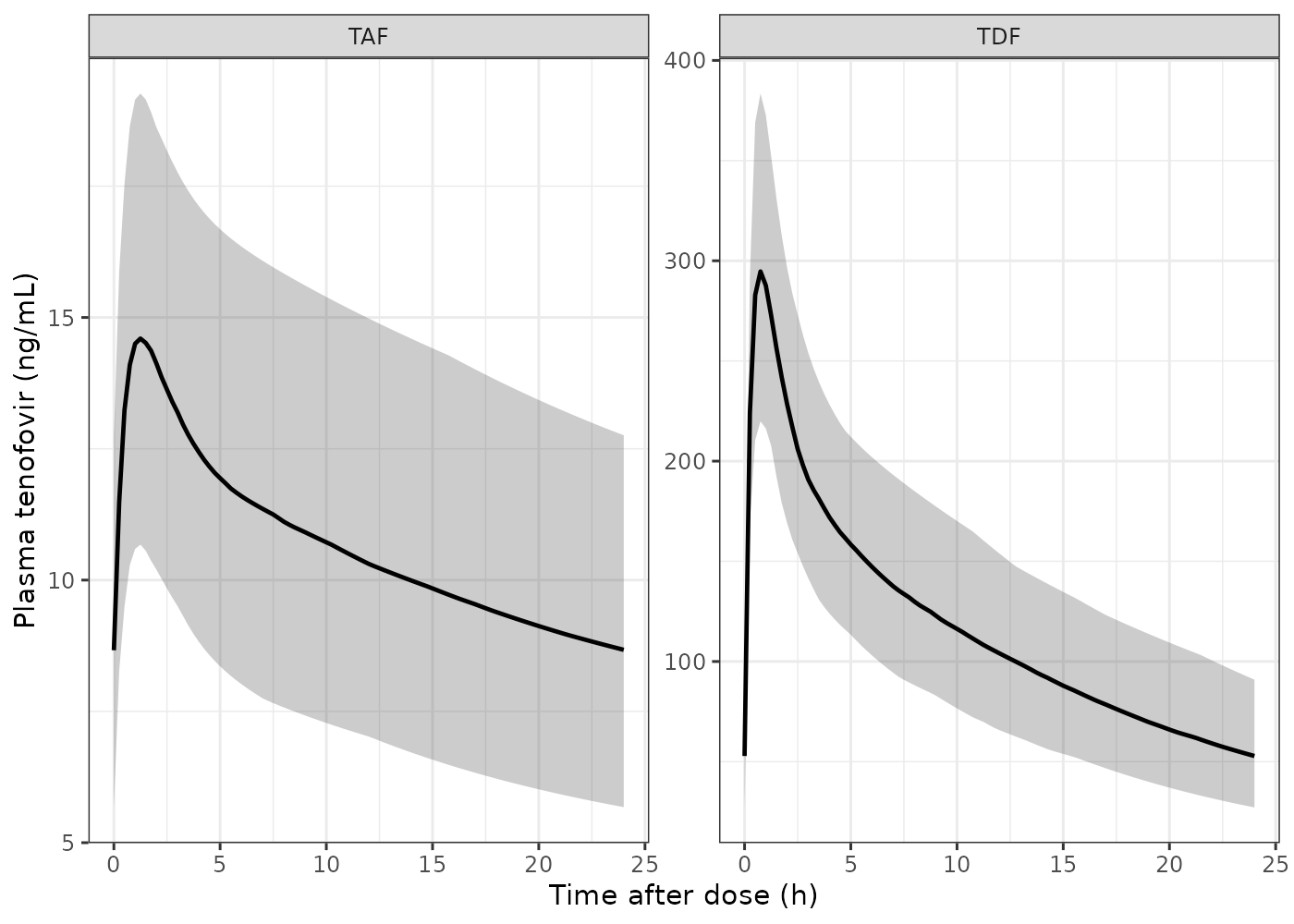
Simulated steady-state tenofovir concentration-time profiles over one dosing interval, 200 subjects per arm. Median and 5th / 95th percentiles, the same summary shown in the visual predictive check of Kawuma 2023 Figure 3. Note the free y scales: TDF exposure is about ten-fold higher.
cohort_conc <- PKNCA::PKNCAconc(
  cohort, conc ~ time | arm + id, concu = "ng/mL", timeu = "h"
)
cohort_dose <- cohort |>
  distinct(arm, id) |>
  mutate(
    dose = if_else(arm == "TDF", tfv_tdf300, tfv_taf25),
    time = start_ss
  )
cohort_dose_obj <- PKNCA::PKNCAdose(
  cohort_dose, dose ~ time | arm + id, doseu = "mg"
)

cohort_nca <- PKNCA::pk.nca(
  PKNCA::PKNCAdata(cohort_conc, cohort_dose_obj, intervals = intervals)
)

cohort_summary <- as.data.frame(cohort_nca$result) |>
  filter(PPTESTCD %in% c("auclast", "cmax", "cmin", "tmax")) |>
  group_by(arm, PPTESTCD) |>
  summarise(
    median = stats::median(PPORRES),
    p05 = stats::quantile(PPORRES, 0.05),
    p95 = stats::quantile(PPORRES, 0.95),
    .groups = "drop"
  )

knitr::kable(
  cohort_summary |>
    rename("Arm" = arm, "Parameter" = PPTESTCD, "Median" = median,
           "5th percentile" = p05, "95th percentile" = p95),
  digits = 2,
  caption = "Simulated steady-state NCA parameters by arm (AUC0-24 and concentrations in ng*h/mL and ng/mL, tmax in h)."
)| Arm | Parameter | Median | 5th percentile | 95th percentile |
|---|---|---|---|---|
| TAF | auclast | 255.81 | 171.67 | 414.90 |
| TAF | cmax | 14.64 | 10.40 | 21.65 |
| TAF | cmin | 8.61 | 5.60 | 14.55 |
| TAF | tmax | 1.25 | 1.25 | 1.25 |
| TDF | auclast | 2837.13 | 1903.79 | 4606.10 |
| TDF | cmax | 290.24 | 210.34 | 391.55 |
| TDF | cmin | 52.51 | 28.03 | 102.34 |
| TDF | tmax | 0.75 | 0.75 | 0.75 |
med_auc <- cohort_summary |>
  filter(PPTESTCD == "auclast") |>
  select(arm, median) |>
  tidyr::pivot_wider(names_from = arm, values_from = median)

tdf_taf_ratio <- med_auc$TDF / med_auc$TAF
tdf_taf_ratio
#> [1] 11.09088

stopifnot(
  # Kawuma 2023 Figure 1 legend: "when given as TDF, tenofovir in the plasma
  # is more than 10-fold higher than when TAF is administered".
  tdf_taf_ratio > 10
)
The observed AUC0-24h in the study itself (Kawuma 2023 Table 3,
“Observed (this study)”) was 3022 ng*h/mL on TDF and 267.1
ng*h/mL on TAF – a ratio of 11.3 – against the 11.1-fold
ratio simulated here at the cohort weight distribution.
Assumptions and deviations
Doses are tenofovir-equivalent amounts, not prodrug amounts. A user dosing this model with
amt = 300for TDF, oramt = 25for TAF, will over-predict exposure by roughly the molecular-weight ratio. Use 136 mg and 15 mg, or convert with the molecular weights given above.A TAF dose requires two dose records, into
depot2anddepot3, both carrying the same tenofovir-equivalent amount. Thef()terms split that amount; giving only one record delivers only that pathway’s share.Between-occasion variability is encoded with explicit per-occasion etas. rxode2 has no NONMEM-style
| occasionrandom-effect level, so the BOV onF_TDF,Ka_TDFandKa_TAFis expanded into one eta per occasion, selected by theOCCindicators. Kawuma 2023 defines exactly two occasions (the unobserved dose the day before the visit, and the observed dose on the day of the visit), so two are encoded, with the second variance fixed to the first – the equivalent of NONMEM’s$OMEGA BLOCK(1) SAME. Because the occasion effect enters as an indicator-weighted sum rather than as a bare term, rxode2 emitssome etas defaulted to non-mu referencedon every solve. This is expected and affects only mu-referencing speed-ups in a future estimation run; simulation, which is what this model is shipped for, is unaffected. PassingOCC = 0(as every simulation here does) zeroes all indicators and removes the between-occasion contribution, reproducing the authors’ own simulation setting.The variance scale is the SD convention. Table 2 footnote b states
CV% = sqrt(omega^2) * 100, so theini()variances are(CV/100)^2. Using the more commonlog(1 + CV^2)conversion instead would inflate the BOV onKa_TDF(114.5% CV) substantially.t1/2_TAF-Slowis fixed, and only weakly identified. The authors estimated it first, found it poorly identifiable, and reported that likelihood profiling gave “only small changes in terms of goodness-of-fit” anywhere in the range 5 to 60 days. They fixed it at 6.83 days, the published intracellular TFV-DP decay half-life. It is encoded here as a fixed first-order rate constantlog(2) / (6.83 x 24)per hour. The sensitivity analysis behind this choice is in the paper’s Table S1 and Figure S4, which were not available (see below); the final fixed value itself is printed in Table 2 of the main text.The model does not reproduce the secondary TAF peak. The Discussion notes that the observed TAF profiles show “after an initial peak at about 1 h postdose, … a secondary peak at about 4 h postdose”, and speculates that it reflects intracellular TAF conversion. The fitted structure releases from the reservoir by a single slow first-order process with a multi-day half-life, which is monotone and cannot produce a secondary peak. This is a property of the published model, not of the encoding.
Age and creatinine clearance were screened and dropped. Neither improved the fit, and no coefficient is published for either, so neither can be encoded. They are recorded in
covariatesDataExcludedto preserve the provenance of the covariate screen. The authors flag the negative renal finding as a limitation, attributing it to the narrow creatinine-clearance range in the cohort and to creatinine not being measured at the time of drug sampling.No variability on Vc, Q, Vp, F_TAF or Frac_TAF-Fast. Table 2 leaves those variability cells blank, and the Results state that within the TAF arm the model “did not support the estimation of any variability (BOV or BSV) on the bioavailability parameter”. No variance is invented for them.
Race and ethnicity are not reported. Table 1 gives sex, age, weight, height and creatinine clearance only, so
population$race_ethnicityrecords the absence rather than a distribution. The weight distribution used for the cohort simulation above is a log-normal matched to the published median and IQR, not a resampling of the actual 41 participants, whose individual covariates were not available.Fat-free mass was tested and rejected. The authors report that FFM scaling did not improve the model over no allometry (dOFV = -3.80) whereas total body weight did (dOFV = -18), so total body weight is the size descriptor encoded here.
Supplementary material not obtained
The article’s Supporting Information – Figures S1-S4 (raw data and
goodness-of-fit plots, plus the t1/2_TAF-Slow sensitivity
figure), Table S1 (the t1/2_TAF-Slow sensitivity analysis),
a NONMEM control stream deposited as PSP4-12-821-s007.mod,
and the concentration dataset PSP4-12-821-s006.xlsx – could
not be retrieved when this model was built: PMC serves supplementary
files only through an interactive browser challenge, and the Wiley
landing page refused access.
No parameter used by this model comes from those files: every
structural element is specified in the Methods and the Figure 2 legend,
and every final estimate is printed in Table 2 of the main text. The
control stream would be a useful independent confirmation of the
encoding, and is worth retrieving if a reviewer wants one; note that a
control stream’s $THETA block holds initial, not final,
estimates, so Table 2 would remain the authoritative source either
way.