Tacrolimus minimal PBPK in living-donor liver transplantation (Itohara 2019)
Source:vignettes/articles/Itohara_2019_tacrolimus.Rmd
Itohara_2019_tacrolimus.RmdModel and source
- Citation: Itohara K, Yano I, Tsuzuki T, Uesugi M, Nakagawa S, Yonezawa A, Okajima H, Kaido T, Uemoto S, Matsubara K. A Minimal Physiologically-Based Pharmacokinetic Model for Tacrolimus in Living-Donor Liver Transplantation: Perspectives Related to Liver Regeneration and the Cytochrome P450 3A5 (CYP3A5) Genotype. CPT Pharmacometrics Syst Pharmacol. 2019;8(8):587-595. doi:10.1002/psp4.12420. Model equations from main-text Eq. 1 and Supplementary Information Eq. 1-7; drug and system parameters from Table S2; final NONMEM control stream from the Supplementary Information. The absorption rate constant (not reported) is taken from Ji E, Kim MG, Oh JM. Ther Clin Risk Manag. 2018;14:2119-2126, doi:10.2147/TCRM.S184376 (Ji_2018_tacrolimus.R).
- Description: PBPK (minimal, Simcyp v17 parameterisation re-encoded in NONMEM 7.2). Tacrolimus whole-blood pharmacokinetics in adult Japanese living-donor liver transplant (LDLT) recipients during the first postoperative month. One-compartment disposition (Vd = 1.29 L/kg) with first-order oral absorption; clearance is a well-stirred hepatic extraction of an enzyme-abundance intrinsic clearance (CYP3A4 + CYP3A5, 13-O-desmethylation and 12-hydroxylation) scaled by a regenerating graft liver (60% of standard size at surgery, half-recovery in one postoperative day). Oral bioavailability is Fa x Fg x Fh with a Qgut gut-wall model whose CYP3A Michaelis-Menten extraction saturates on the portal-vein concentration. Hepatic CYP3A5 follows the DONOR (graft) genotype and intestinal CYP3A5 follows the RECIPIENT genotype. Deterministic given covariates (the source control stream fixes both etas to zero).
- Article: https://doi.org/10.1002/psp4.12420 (open access; the Supplementary Information holds Table S2, the Simcyp equations and the final NONMEM control stream)
Itohara et al. built a minimal PBPK model of tacrolimus in Simcyp v17 and re-encoded it in NONMEM so that a time-varying graft-liver size could be added. The structure is a one-compartment model with first-order oral absorption; the physiology lives in how clearance and bioavailability are computed:
- Clearance is a well-stirred hepatic extraction (SI Eq. 4 and 7) of an intrinsic clearance built from recombinant-CYP kinetics for two CYP3A4 and two CYP3A5 pathways (13-O-desmethylation and 12-hydroxylation), scaled by hepatic enzyme abundance, microsomal protein and liver weight (SI Eq. 1).
-
Liver regeneration (main-text Eq. 1, the selected
model): the graft is 60% of the recipient’s standard liver size at
surgery and recovers hyperbolically with a half-recovery time of one
postoperative day,
LW = (GR + (1 - GR) / (1 + 1/POD)) * LWstd. -
Bioavailability is
F = Fa x Fg x Fh, withFadesignated 0.6 and a Qgut gut-wall model (SI Eq. 5) whose CYP3A Michaelis-Menten extraction saturates on the portal-vein concentration. -
Genotype: hepatic CYP3A5 follows the donor
(graft) genotype and intestinal CYP3A5 the recipient genotype.
The paper’s four groups are L*1/I*1, L*1/I*3, L*3/I*1 and L*3/I*3 (L =
graft liver, I = recipient intestine, *1 = CYP3A5*1 carrier, *3 =
CYP3A5*3/*3), i.e.
CYP3A5_EXPR_DONORandCYP3A5_EXPRin this model.
Population
Model building used 26 adult LDLT recipients at Kyoto University Hospital (December 2013 - January 2016; mean age 53.5 years, mean weight 66.6 kg, mean hematocrit 25.5%) with routine TDM concentrations during the initial intravenous infusion and oral troughs. Verification used 272 adult LDLT recipients (July 2004 - June 2011; mean age 52.2 years, mean weight 60.1 kg) with trough concentrations over the first 28 postoperative days. Donor CYP3A5 *3/*3 / *1/*3 / *1/*1 counts were 14 / 11 / 1 (building) and 166 / 92 / 14 (verification); recipient counts were 15 / 9 / 2 and 171 / 88 / 13 (Table S1). All simulations in the paper used 100 Simcyp Japanese virtual adults per genotype combination on the 2013 Kyoto protocol: intravenous tacrolimus 1.25 ug/h/kg for 12 h, then 0.83 ug/h/kg, switched on POD 3 to oral 0.04 mg/kg/day.
The same information is available programmatically via
readModelDb("Itohara_2019_tacrolimus_pbpk")()$population.
Source trace
Every ini() value carries an in-file comment pointing to
its source; the table collects them.
| Equation / parameter | Value | Source location |
|---|---|---|
Liver regeneration
f_regen = gr + (1 - gr) POD/(POD + 1)
|
n/a | Main-text Eq. 1 (selected; lowest SQE, P < 0.001 vs Eq. 2-4);
control stream LV
|
gr |
0.6 | Methods ‘GR was assumed to be 60%’; control stream
LVD=LVR*0.6
|
| Hepatic CLint (SI Eq. 1) | n/a | SI Eq. 1; control stream CLIL (constant 1080 = liver
density g/L, 0.00006 = 1e-6 x 60) |
| Well-stirred CL and Fh | n/a | SI Eq. 4, 7; control stream TVCL, FH
|
| Gut CLint and Fg (SI Eq. 2, 5) with two-step saturable refinement | n/a | SI Eq. 2, 5; control stream CLIG, INI,
CLIGI, CPV, CLIGM,
FGA
|
F = Fa x Fg x Fh |
n/a | SI ‘Bioavailability F is the product of Fa, Fh and Fg’; control
stream F1
|
Vd = vc x WT |
n/a | SI Eq. 6 |
lka |
log(4.48) | Not in the paper; Ji 2018 Table 2 (see Assumptions) |
fa |
0.6 | Results ‘PBPK modeling’ (smallest RMSE) and ‘Simulation’ |
lvc |
log(1.29) L/kg | Table S2 ‘Vb’; Methods |
fu, bpr, fu_gut
|
0.013, 35, 1 | Table S2 |
isef |
0.24 | Table S2 (all pathways) |
vmax_*, km_* (8 values) |
8, 0.21; 0.6, 0.29; 17, 0.21; 1.4, 0.35 | Table S2 (Dai 2006); control stream CLIL
|
abund_cyp3a4_liver,
abund_cyp3a5_liver
|
93, 17 pmol/mg | Table S2; Methods ‘PBPK model development’ |
mppgl_vliver |
56.04 | Back-solved (see below) |
qco |
251 L/h | Back-solved (see below) |
fq_liver_*, fq_pv_*
|
0.255 / 0.280, 0.19 / 0.215 | Control stream B, C
|
qgut |
11.4 L/h | Table S2 ‘Qgut’ |
abund_cyp3a4_gut, abund_cyp3a5_gut
|
76585, 20283 pmol | Back-solved (see below) |
expSd |
0.3162 | Control stream $SIGMA 0.1,
Y=F*EXP(EPS(1))
|
| No IIV | n/a | Control stream $OMEGA 0 FIXED 0 FIXED
|
Typical-value simulation
All validation below uses a typical 60 kg male recipient (the verification cohort’s mean weight; the cardiac output was back-solved for the male hepatic-flow fraction) on the paper’s standard protocol, one subject per genotype combination. The model has no random effects, so these are exact typical-value predictions.
mod <- readModelDb("Itohara_2019_tacrolimus_pbpk")

genotypes <- tibble::tibble(
  geno = c("L*1/I*1", "L*1/I*3", "L*3/I*1", "L*3/I*3"),
  CYP3A5_EXPR_DONOR = c(1, 1, 0, 0),
  CYP3A5_EXPR = c(1, 0, 1, 0)
)

# Kyoto 2013 protocol: IV 1.25 ug/h/kg for 12 h, 0.83 ug/h/kg until POD 3,
# then oral 0.04 mg/kg/day as 0.02 mg/kg every 12 h. Doses in mg, time in h.
protocol_events <- function(id, wt, sexf, ld, ir, obs_times) {
  iv <- data.frame(
    time = c(0, 12),
    amt = c(1.25e-3 * wt * 12, 0.83e-3 * wt * 60),
    rate = c(1.25e-3 * wt, 0.83e-3 * wt),
    evid = 1L, cmt = "central"
  )
  po <- data.frame(
    time = seq(72, 28 * 24 - 12, by = 12),
    amt = 0.02 * wt, rate = 0, evid = 1L, cmt = "depot"
  )
  obs <- data.frame(time = obs_times, amt = 0, rate = 0, evid = 0L, cmt = "central")
  dplyr::bind_rows(iv, po, obs) |>
    dplyr::arrange(time, dplyr::desc(evid)) |>
    dplyr::mutate(
      id = id, WT = wt, SEXF = sexf, POD = time / 24,
      CYP3A5_EXPR_DONOR = ld, CYP3A5_EXPR = ir
    )
}

obs_grid <- seq(0, 28 * 24, by = 1)
ev_typ <- dplyr::bind_rows(lapply(seq_len(nrow(genotypes)), function(i) {
  protocol_events(i, 60, 0, genotypes$CYP3A5_EXPR_DONOR[i], genotypes$CYP3A5_EXPR[i], obs_grid) |>
    dplyr::mutate(geno = genotypes$geno[i])
}))
stopifnot(!anyDuplicated(ev_typ[ev_typ$evid == 0, c("id", "time")]))

# The model has no random effects, so rxode2's "multi-subject simulation
# without 'omega'" note below is expected: the subjects differ only in
# covariates.
sim_typ <- rxode2::rxSolve(mod, events = ev_typ, keep = "geno", returnType = "data.frame")
#> Warning: multi-subject simulation without without 'omega'
stopifnot(all(is.finite(sim_typ$Cc)))
Back-solved inputs reproduce the paper’s hepatic and gut outputs
Four $INPUT items of the control stream are Simcyp
virtual-population outputs whose values the paper does not print (see
Assumptions). They were back-solved from the paper’s own reported
outputs, so the comparison below is a self-consistency check of
the back-solve, not an independent validation: two hepatic
values (mppgl_vliver, qco) against six printed
hepatic outputs, and two gut abundances against the two printed
Fg values.
at_time <- function(t) {
  sim_typ |>
    dplyr::filter(abs(time - t) < 1e-9) |>
    dplyr::distinct(geno, .keep_all = TRUE)
}
cl_pod <- function(pod) {
  # CL for a given POD from the model's own equations (deterministic).
  ev <- protocol_events(1, 60, 0, 1, 0, pod * 24)
  ev <- ev[ev$evid == 0, ]
  ev <- dplyr::bind_rows(ev, dplyr::mutate(ev, id = 2, CYP3A5_EXPR_DONOR = 0))
  s <- rxode2::rxSolve(mod, events = ev, returnType = "data.frame")
  stats::setNames(s$cl, c("L*1", "L*3"))
}
cl0 <- cl_pod(0)
#> Warning: multi-subject simulation without without 'omega'
cl30 <- cl_pod(30)
#> Warning: multi-subject simulation without without 'omega'
end <- at_time(660) # last oral dose (POD 27.5): F evaluated with its dose and trough

hep <- tibble::tribble(
  ~quantity, ~published, ~model,
  "CL, L*1, POD 0 (L/h)", 0.975, cl0[["L*1"]],
  "CL, L*3, POD 0 (L/h)", 0.729, cl0[["L*3"]],
  "CL, L*1, POD 30 (L/h)", 1.59, cl30[["L*1"]],
  "CL, L*3, POD 30 (L/h)", 1.19, cl30[["L*3"]],
  "Fh, L*1", 0.979, end$fh[end$geno == "L*1/I*1"],
  "Fh, L*3", 0.985, end$fh[end$geno == "L*3/I*3"],
  "Fg, I*1 (mean over L)", 0.153, mean(end$fg[end$geno %in% c("L*1/I*1", "L*3/I*1")]),
  "Fg, I*3 (mean over L)", 0.227, mean(end$fg[end$geno %in% c("L*1/I*3", "L*3/I*3")])
) |>
  dplyr::mutate(pct_diff = 100 * (model / published - 1))

hep |>
  dplyr::mutate(model = signif(model, 4), pct_diff = round(pct_diff, 1)) |>
  dplyr::rename(
    "Quantity" = quantity, "Published" = published,
    "Model" = model, "Difference (%)" = pct_diff
  ) |>
knitr::kable(caption = "Back-solve self-consistency (Results 'Simulation'; Discussion).")| Quantity | Published | Model | Difference (%) |
|---|---|---|---|
| CL, L*1, POD 0 (L/h) | 0.975 | 0.9904 | 1.6 |
| CL, L*3, POD 0 (L/h) | 0.729 | 0.7174 | -1.6 |
| CL, L*1, POD 30 (L/h) | 1.590 | 1.6130 | 1.5 |
| CL, L*3, POD 30 (L/h) | 1.190 | 1.1720 | -1.5 |
| Fh, L*1 | 0.979 | 0.9748 | -0.4 |
| Fh, L*3 | 0.985 | 0.9817 | -0.3 |
| Fg, I*1 (mean over L) | 0.153 | 0.1530 | 0.0 |
| Fg, I*3 (mean over L) | 0.227 | 0.2270 | 0.0 |
Figure 6: CL, F and CL/F over the first postoperative month
# F depends on the dose amount and the blood level at the dose, so it is read
# at the oral dose times (every 12 h from POD 3), where f(depot) applies.
fig6 <- sim_typ |>
  dplyr::filter(time >= 72, time < 28 * 24, abs(time %% 12) < 1e-9) |>
  dplyr::mutate(POD = time / 24, `CL/F (L/h)` = cl / f_oral) |>
  dplyr::select(geno, POD, `CL (L/h)` = cl, `F` = f_oral, `CL/F (L/h)`) |>
  tidyr::pivot_longer(-c(geno, POD), names_to = "quantity")

ggplot(fig6, aes(POD, value, colour = geno, linetype = geno)) +
  geom_line() +
  facet_wrap(~quantity, ncol = 1, scales = "free_y") +
  labs(
    x = "Postoperative day", y = NULL, colour = "Genotype", linetype = "Genotype",
    title = "Typical CL, F and CL/F after LDLT",
    caption = "Replicates Figure 6 of Itohara 2019 (typical 60 kg male, oral doses from POD 3)."
  )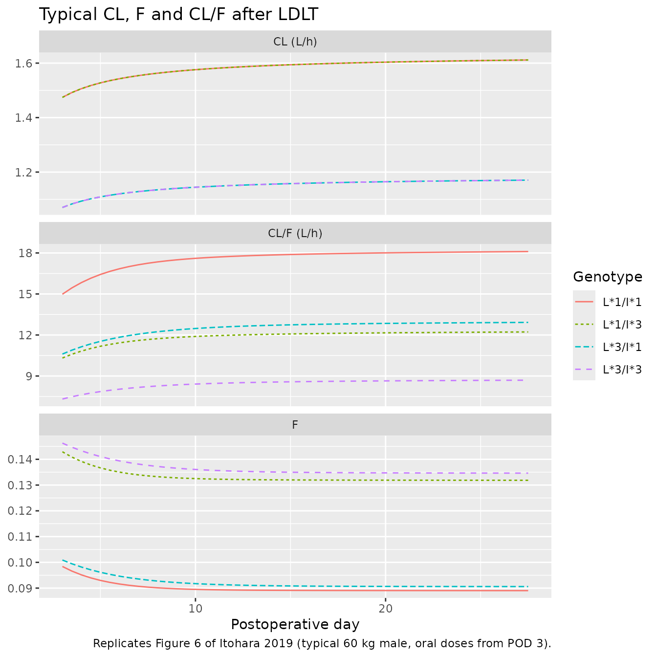
CL depends only on the graft genotype and F almost only on the
recipient genotype, so pairs of lines overlap in those panels. Before
the first oral dose the model has no dose amount for the saturable gut
term, so F is shown from POD 3.
f_tab <- tibble::tribble(
  ~geno, ~F_pub, ~CLF_pub,
  "L*1/I*1", 0.090, 17.0,
  "L*1/I*3", 0.131, 11.3,
  "L*3/I*1", 0.090, 11.8,
  "L*3/I*3", 0.131, 7.9
) |>
  dplyr::left_join(
    end |> dplyr::transmute(geno, F_model = f_oral, CLF_model = cl / f_oral),
    by = "geno"
  ) |>
  dplyr::mutate(
    F_pct = 100 * (F_model / F_pub - 1),
    CLF_pct = 100 * (CLF_model / CLF_pub - 1)
  )

f_tab |>
  dplyr::mutate(dplyr::across(c(F_model, CLF_model), \(x) signif(x, 3)),
                dplyr::across(c(F_pct, CLF_pct), \(x) round(x, 1))) |>
  dplyr::rename(
    "Genotype" = geno, "F, published" = F_pub, "F, model" = F_model,
    "F diff (%)" = F_pct, "CL/F published (L/h)" = CLF_pub,
    "CL/F model (L/h)" = CLF_model, "CL/F diff (%)" = CLF_pct
  ) |>
knitr::kable(caption = "End-of-month F and CL/F (Results 'Simulation'; the paper prints one F per intestinal genotype).")| Genotype | F, published | CL/F published (L/h) | F, model | CL/F model (L/h) | F diff (%) | CL/F diff (%) |
|---|---|---|---|---|---|---|
| L1/I1 | 0.090 | 17.0 | 0.0890 | 18.10 | -1.1 | 6.5 |
| L1/I3 | 0.131 | 11.3 | 0.1320 | 12.20 | 0.6 | 8.2 |
| L3/I1 | 0.090 | 11.8 | 0.0906 | 12.90 | 0.7 | 9.5 |
| L3/I3 | 0.131 | 7.9 | 0.1350 | 8.69 | 2.8 | 10.0 |
# F is Fa x Fg x Fh, all three pinned above: measured |diff| <= 2.8%.
# CL/F runs 6-10% high in every group: the paper reports the MEDIAN of the
# per-subject CL/F of 100 virtual subjects with log-normal CYP abundances,
# while CL and F were matched to its MEAN CL and median F; the gate allows 15%.
stopifnot(
  nrow(f_tab) == 4L, all(is.finite(f_tab$F_model)),
  all(abs(f_tab$F_pct) < 5),
  all(abs(f_tab$CLF_pct) < 15)
)
Figure 4: blood concentrations immediately after LDLT
sim_typ |>
  dplyr::filter(time <= 7 * 24) |>
  ggplot(aes(time / 24, Cc, colour = geno)) +
  geom_line() +
  geom_vline(xintercept = 3, linetype = "dashed", colour = "grey50") +
  labs(
    x = "Postoperative day", y = "Whole-blood tacrolimus (ng/mL)",
    colour = "Genotype",
    title = "Typical concentration on the standard protocol",
    caption = "Replicates the median lines of Figure 4 of Itohara 2019.\nIV until POD 3 (dashed), then oral 0.04 mg/kg/day."
  )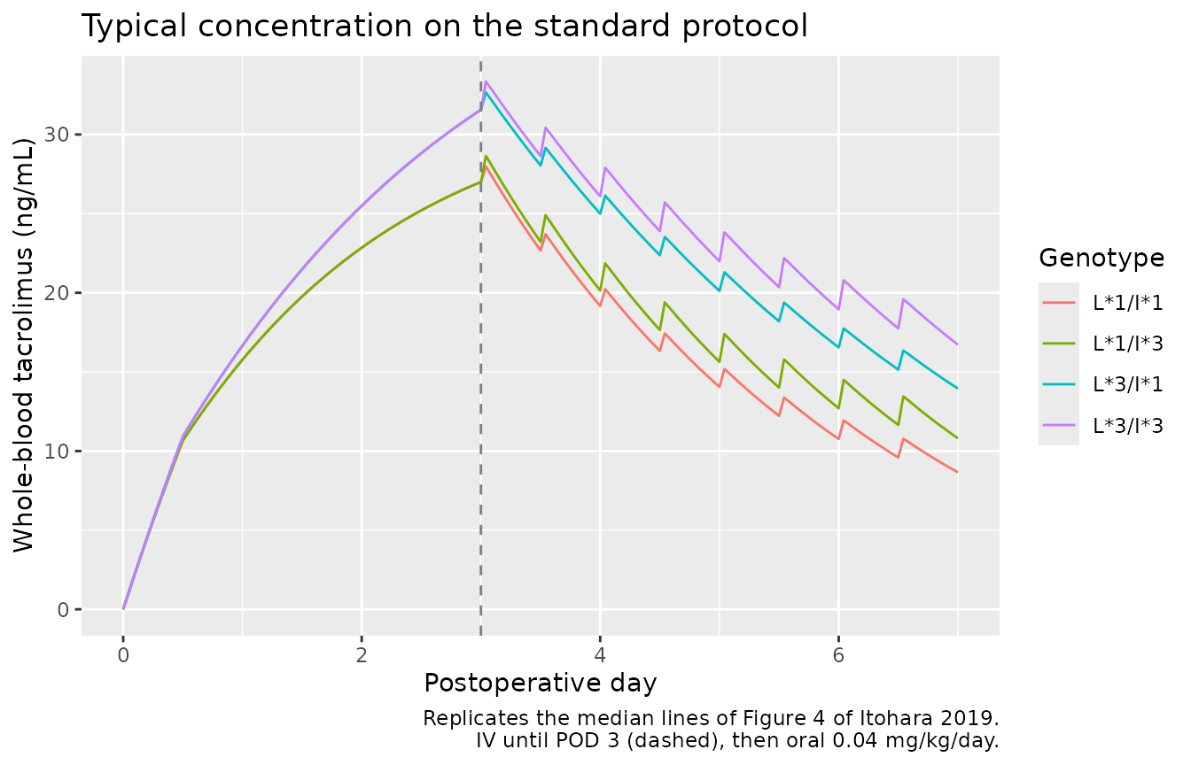
Figure 5: trough concentration/dose ratios
The paper verified the model against observed trough C/D ratios ((ng/mL)/(mg/kg/day)) in three weekly windows and printed the predicted medians for POD 22-28: 102, 155, 167 and 244 for L*1/I*1, L*1/I*3, L*3/I*1 and L*3/I*3. The model’s only between-subject inputs are weight and sex, so the virtual cohort below (100 per genotype, the paper’s number) varies those alone; weight is drawn from the verification cohort’s mean (SD) of 60.1 (12.3) kg and half the subjects are female (sex was not reported).
set.seed(20190828)
n_per <- 100L
cohort <- tidyr::expand_grid(genotypes, k = seq_len(n_per)) |>
  dplyr::mutate(
    id = seq_len(dplyr::n()),
    WT = pmin(pmax(stats::rnorm(dplyr::n(), 60.1, 12.3), 35), 100),
    SEXF = stats::rbinom(dplyr::n(), 1, 0.5)
  )
trough_times <- seq(72 + 11.99, 28 * 24, by = 12)
ev_coh <- dplyr::bind_rows(lapply(seq_len(nrow(cohort)), function(i) {
  protocol_events(
    cohort$id[i], cohort$WT[i], cohort$SEXF[i],
    cohort$CYP3A5_EXPR_DONOR[i], cohort$CYP3A5_EXPR[i], trough_times
  ) |>
    dplyr::mutate(geno = cohort$geno[i])
}))
sim_coh <- rxode2::rxSolve(mod, events = ev_coh, keep = c("geno", "WT"), returnType = "data.frame")
#> Warning: multi-subject simulation without without 'omega'

cd <- sim_coh |>
  dplyr::mutate(
    POD = time / 24,
    window = cut(POD, c(8, 15, 22, 29), right = FALSE, labels = c("POD 8-14", "POD 15-21", "POD 22-28")),
    cd = Cc / 0.04
  ) |>
  dplyr::filter(!is.na(window))

ggplot(cd, aes(geno, cd)) +
  geom_boxplot(outlier.size = 0.5) +
  facet_wrap(~window) +
  labs(
    x = NULL, y = "Trough C/D ((ng/mL)/(mg/kg/day))",
    title = "Trough C/D ratio by genotype and week",
    caption = paste(
      "Replicates the predicted boxes of Figure 5 of Itohara 2019",
      "(spread from weight and sex only)."
    )
  ) +
  theme(axis.text.x = element_text(angle = 30, hjust = 1))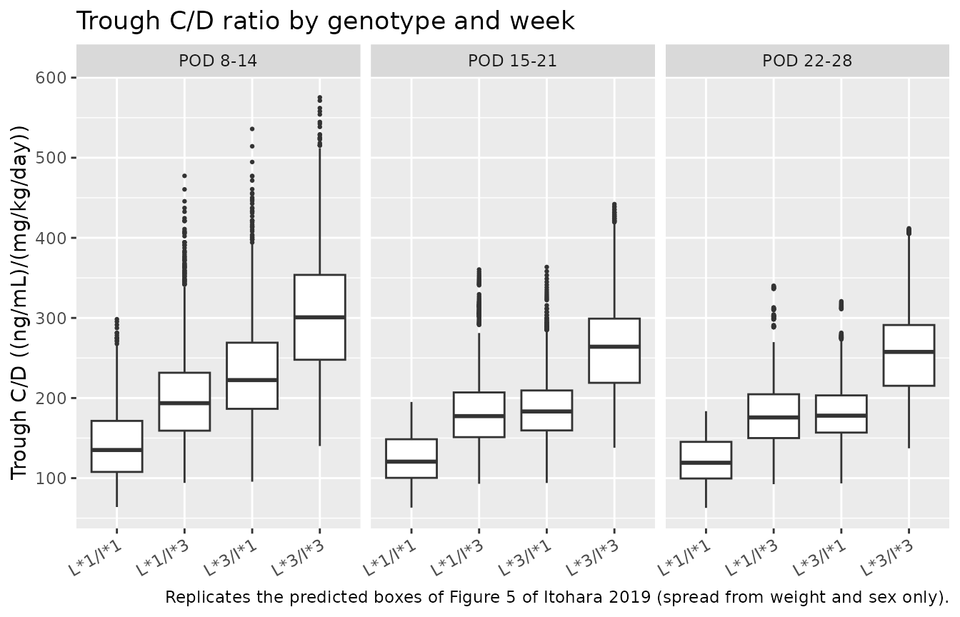
cd_tab <- cd |>
  dplyr::filter(window == "POD 22-28") |>
  dplyr::group_by(geno) |>
  dplyr::summarise(cd_model = stats::median(cd), .groups = "drop") |>
  dplyr::left_join(
    tibble::tibble(geno = genotypes$geno, cd_pub = c(102, 155, 167, 244)),
    by = "geno"
  ) |>
  dplyr::mutate(pct_diff = 100 * (cd_model / cd_pub - 1))

cd_tab |>
  dplyr::mutate(cd_model = round(cd_model), pct_diff = round(pct_diff, 1)) |>
  dplyr::rename(
    "Genotype" = geno, "Median C/D, model" = cd_model,
    "Median C/D, published" = cd_pub, "Difference (%)" = pct_diff
  ) |>
knitr::kable(caption = "Predicted median trough C/D, POD 22-28 (Results 'Model verification').")| Genotype | Median C/D, model | Median C/D, published | Difference (%) |
|---|---|---|---|
| L1/I1 | 119 | 102 | 16.9 |
| L1/I3 | 176 | 155 | 13.4 |
| L3/I1 | 178 | 167 | 6.6 |
| L3/I3 | 258 | 244 | 5.6 |
# Centre-of-distribution gate: the ordering
# L*1/I*1 < L*1/I*3 ~ L*3/I*1 < L*3/I*3 is structural and the medians must lie
# within 25% of the paper's (measured +6% to +17%; the L*1 groups run highest,
# see Assumptions). Weight and sex barely move the median, so the bound has
# headroom on any cohort draw.
stopifnot(
  nrow(cd_tab) == 4L,
  all(abs(cd_tab$pct_diff) < 25),
  cd_tab$cd_model[cd_tab$geno == "L*1/I*1"] < cd_tab$cd_model[cd_tab$geno == "L*3/I*3"]
)
Table 1: genotype-guided starting doses
The paper derived three doses from the final model: an intravenous
loading rate that brings the concentration to 15 ng/mL at 12 h, a
maintenance rate that holds 15 ng/mL from POD 0.5, and an oral daily
dose that holds a 10 ng/mL trough at POD 3. They are recomputed below
for the typical 60 kg male. The oral dose is found by root-finding
because the saturable gut makes F depend on the dose; it is
the steady-state trough with POD held at 3.
one_subject <- function(ld, ir, ev) {
  ev |> dplyr::mutate(id = 1, WT = 60, SEXF = 0, CYP3A5_EXPR_DONOR = ld, CYP3A5_EXPR = ir)
}
# Loading: concentration at 12 h per 1 ug/h/kg is linear in the rate.
load_rate <- function(ld, ir) {
  ev <- data.frame(
    time = c(0, 12), amt = c(1e-3 * 60 * 12, 0), rate = c(1e-3 * 60, 0),
    evid = c(1L, 0L), cmt = "central"
  ) |>
    one_subject(ld = ld, ir = ir) |>
    dplyr::mutate(POD = time / 24)
  c12 <- rxode2::rxSolve(mod, events = ev, returnType = "data.frame")$Cc
  15 / c12
}
# Maintenance: CL at POD 0.5 x 15 ng/mL, per kg.
maint_rate <- function(ld, ir) {
  ev <- data.frame(time = 12, amt = 0, rate = 0, evid = 0L, cmt = "central") |>
    one_subject(ld = ld, ir = ir) |>
    dplyr::mutate(POD = 0.5)
  rxode2::rxSolve(mod, events = ev, returnType = "data.frame")$cl * 15 / 60
}
# Oral: steady-state trough at POD 3 (30 days of q12h dosing, POD frozen).
trough_pod3 <- function(dose_mgkgday, ld, ir) {
  dose_t <- seq(0, 30 * 24 - 12, by = 12)
  ev <- dplyr::bind_rows(
    data.frame(time = dose_t, amt = dose_mgkgday / 2 * 60, rate = 0, evid = 1L, cmt = "depot"),
    data.frame(time = 30 * 24, amt = 0, rate = 0, evid = 0L, cmt = "central")
  ) |>
    one_subject(ld = ld, ir = ir) |>
    dplyr::mutate(POD = 3)
  s <- rxode2::rxSolve(mod, events = ev, returnType = "data.frame")
  s$Cc[nrow(s)]
}
oral_dose <- function(ld, ir) {
  stats::uniroot(function(d) trough_pod3(d, ld, ir) - 10, c(0.005, 0.3), tol = 1e-6)$root
}

tab1 <- genotypes |>
  dplyr::rowwise() |>
  dplyr::mutate(
    load = load_rate(CYP3A5_EXPR_DONOR, CYP3A5_EXPR),
    maint = maint_rate(CYP3A5_EXPR_DONOR, CYP3A5_EXPR),
    oral = oral_dose(CYP3A5_EXPR_DONOR, CYP3A5_EXPR)
  ) |>
  dplyr::ungroup() |>
  dplyr::mutate(ratio = oral / (maint * 24 / 1000)) |>
  dplyr::left_join(
    tibble::tibble(
      geno = genotypes$geno,
      load_pub = c(1.41, 1.41, 1.31, 1.31),
      maint_pub = c(0.309, 0.309, 0.230, 0.230),
      oral_pub = c(0.0662, 0.0446, 0.0468, 0.0306)
    ),
    by = "geno"
  )

tab1 |>
  dplyr::transmute(
    geno,
    load = sprintf("%.2f (%.2f)", load, load_pub),
    maint = sprintf("%.3f (%.3f)", maint, maint_pub),
    oral = sprintf("%.4f (%.4f)", oral, oral_pub),
    ratio = sprintf("%.2f", ratio)
  ) |>
  dplyr::rename(
    "Genotype" = geno,
    "Loading, ug/h/kg: model (paper)" = load,
    "Maintenance at POD 0.5, ug/h/kg: model (paper)" = maint,
    "Oral at POD 3, mg/kg/day: model (paper)" = oral,
    "Oral / IV maintenance" = ratio
  ) |>
knitr::kable(caption = "Recomputed Table 1 of Itohara 2019 (typical 60 kg male).")| Genotype | Loading, ug/h/kg: model (paper) | Maintenance at POD 0.5, ug/h/kg: model (paper) | Oral at POD 3, mg/kg/day: model (paper) | Oral / IV maintenance |
|---|---|---|---|---|
| L1/I1 | 1.74 (1.41) | 0.302 (0.309) | 0.0697 (0.0662) | 9.62 |
| L1/I3 | 1.74 (1.41) | 0.302 (0.309) | 0.0487 (0.0446) | 6.72 |
| L3/I1 | 1.70 (1.31) | 0.219 (0.230) | 0.0499 (0.0468) | 9.50 |
| L3/I3 | 1.70 (1.31) | 0.219 (0.230) | 0.0348 (0.0306) | 6.63 |
tab1_pct <- with(tab1, 100 * c(maint / maint_pub - 1, oral / oral_pub - 1))
# Deterministic. Maintenance -2 to -5% and oral +5 to +14% measured. The
# loading rate is a known deviation (see below) and is not gated.
stopifnot(length(tab1_pct) == 8L, all(is.finite(tab1_pct)), all(abs(tab1_pct) < 20))
The maintenance and oral doses agree with Table 1 to within 14%. The
loading rate does not: the model needs about 1.70-1.74 ug/h/kg against
the paper’s 1.31-1.41. With Vd = 1.29 L/kg (Table S2, SI
Eq. 6), raising the blood concentration to 15 ng/mL within 12 h takes at
least 15 x 1.29 / 12 = 1.61 ug/h/kg even with no
elimination, so the printed loading rates are not reachable with the
paper’s own volume; the paper’s L*1 / L*3 ratio (1.08) is also larger
than its clearances can produce over 12 h. The difference is recorded
here rather than resolved.
PKNCA validation
The paper reports no NCA. PKNCA is used here to confirm, from the
simulated profiles alone, that the apparent oral clearance over the last
dosing interval (POD 27-27.5, effectively steady state) matches the
model’s CL/F and the paper’s end-of-month
CL/F.
sim_nca <- sim_typ |>
  dplyr::filter(!is.na(Cc), time >= 648, time <= 660) |>
  dplyr::select(id, time, Cc, geno)

# Dose in ug so that Dose / AUC (ug / (h x ng/mL)) comes out in L/h.
dose_df <- ev_typ |>
  dplyr::filter(evid == 1, time == 648) |>
  dplyr::mutate(amt = amt * 1000) |>
  dplyr::select(id, time, amt, geno)

conc_obj <- PKNCA::PKNCAconc(sim_nca, Cc ~ time | geno + id)
dose_obj <- PKNCA::PKNCAdose(dose_df, amt ~ time | geno + id)
intervals <- data.frame(
  start = 648, end = 660,
  cmax = TRUE, cmin = TRUE, tmax = TRUE, auclast = TRUE, cl.last = TRUE
)
nca_res <- PKNCA::pk.nca(PKNCA::PKNCAdata(conc_obj, dose_obj, intervals = intervals))

published <- tibble::tibble(geno = f_tab$geno, cl.last = f_tab$CLF_pub)
# ncaParamLabel() has no friendly label for 'cl.last' and warns; the code is
# relabelled below, so only that warning is muffled.
cmp <- withCallingHandlers(
  nlmixr2lib::ncaComparisonTable(
    simulated = nca_res,
    reference = published,
    by = "geno",
    units = c(cl.last = "L/h"),
    tolerance_pct = 20
  ),
  warning = function(w) {
    if (grepl("unknown PKNCA code", conditionMessage(w))) invokeRestart("muffleWarning")
  }
)
cmp$`NCA parameter`[cmp$`NCA parameter` == "cl.last (L/h)"] <- "CL/F = Dose/AUCtau (L/h)"
stopifnot(nrow(cmp) == 4L)
knitr::kable(cmp, caption = "PKNCA over the last dosing interval vs published end-of-month CL/F. * differs from reference by >20%.")| NCA parameter | geno | Reference | Simulated | % diff |
|---|---|---|---|---|
| CL/F = Dose/AUCtau (L/h) | L1/I1 | 17 | 18.2 | +7.0% |
| CL/F = Dose/AUCtau (L/h) | L1/I3 | 11.3 | 12.3 | +8.7% |
| CL/F = Dose/AUCtau (L/h) | L3/I1 | 11.8 | 12.9 | +9.7% |
| CL/F = Dose/AUCtau (L/h) | L3/I3 | 7.9 | 8.71 | +10.2% |
as.data.frame(nca_res) |>
  dplyr::filter(PPTESTCD %in% c("cmax", "cmin", "tmax", "auclast")) |>
  dplyr::select(geno, PPTESTCD, PPORRES) |>
  tidyr::pivot_wider(names_from = PPTESTCD, values_from = PPORRES) |>
  dplyr::mutate(dplyr::across(-geno, \(x) signif(x, 3))) |>
  dplyr::rename(
    "Genotype" = geno, "Cmax (ng/mL)" = cmax, "Cmin (ng/mL)" = cmin,
    "Tmax (h)" = tmax, "AUCtau (h*ng/mL)" = auclast
  ) |>
knitr::kable(caption = "Simulated steady-state exposure on 0.02 mg/kg q12h, POD 27-27.5 (not reported by the paper).")| Genotype | AUCtau (h*ng/mL) | Cmax (ng/mL) | Cmin (ng/mL) | Tmax (h) |
|---|---|---|---|---|
| L1/I1 | 66.0 | 6.14 | 4.89 | 1 |
| L1/I3 | 97.7 | 9.09 | 7.25 | 1 |
| L3/I1 | 92.7 | 8.37 | 7.10 | 1 |
| L3/I3 | 138.0 | 12.40 | 10.60 | 1 |
# Dose/AUCtau must equal the model's own CL/F at steady state (same solve,
# numerical error only; measured < 1%).
cl_last <- as.data.frame(nca_res) |>
  dplyr::filter(PPTESTCD == "cl.last") |>
  dplyr::left_join(f_tab |> dplyr::select(geno, CLF_model), by = "geno")
stopifnot(nrow(cl_last) == 4L, all(abs(cl_last$PPORRES / cl_last$CLF_model - 1) < 0.03))
Assumptions and deviations
-
Absorption rate constant. Itohara 2019 does not
report
ka(theSKAdata item is a Simcyp output), and it cannot be recovered from SI Eq. 3: with the designatedFa = 0.6,Fa = 1 - (1 + ka Tsi / 7)^-7fixes only the productka x Tsi = 0.979. The maintainers ratified usingka = 4.48 1/hfrom the adult LDLT tacrolimus model of Ji 2018 (Ji_2018_tacrolimus, itself fixed from the literature). The paper’s verification data are troughs, sokashapes only the absorption phase and the absorbed-flux part of the saturable gut term; withka = 4.48 1/hthat term is roughly half of the portal-vein concentration at the dose, so a differentkawould shiftFgby several percent. -
Fais a designated constant. The control stream computesFAfromSKAandTSIby SI Eq. 3, but the paper fixedFaat 0.6 for the final model; it is encoded directly andTsiis not needed. -
Back-solved Simcyp inputs. Cardiac output,
microsomal protein per gram of liver, standard liver volume and the
whole-gut CYP3A4 / CYP3A5 abundances are per-subject Simcyp outputs that
the paper does not print. The maintainers back-solved typical values
from the paper’s own outputs (never from Simcyp defaults):
-
qco = 251 L/handmppgl_vliver = 56.04by least squares on the six printed hepatic outputs (CL at POD 0 and 30 and Fh, for L*1 and L*3); only the product of microsomal protein and liver volume is identifiable.qcocorresponds to a hepatic blood flow of 64.0 L/h with the male fraction 0.255; it is applied to both sexes because the sex-specific Simcyp cardiac outputs are not reported, so the female hepatic flow here is 10% higher than the male one (effect on CL < 0.5%). - The gut abundances (
abund_cyp3a4_gut = 76585 pmol,abund_cyp3a5_gut = 20283 pmolfor a CYP3A5*1 recipient) so that the model’s saturableFgat the last oral dose of the standard regimen (POD 27.5, 60 kg male, averaged over graft genotypes) equals the printed 0.227 (I*3) and 0.153 (I*1). The control stream tabulates the saturableFGA, not the linearFG; matching the linear form instead gives 67121 and 19856 pmol and a saturableFgabout 13% above the paper’s. - The printed hepatic CYP3A5 abundance (17 pmol/mg) is the expresser
value; non-expresser grafts carry 0. This is what reproduces both the
L*1 and L*3 clearances with one
mppgl_vliver.
-
-
Km units. Table S2 renders the Km unit as ‘mM’. The
control stream’s unit factor
0.00006 = 1e-6 x 60only works for Km in umol/L, so umol/L is used. - No between-subject variability. The control stream fixes both etas to zero; the paper’s between-subject spread came from Simcyp virtual-population draws (only the hepatic CYP3A4 / CYP3A5 abundance CVs, 81% and 185%, are reported). The model is a typical-value predictor; the Figure 5 cohort varies weight and sex only and is much narrower than the paper’s boxes.
- Weight and liver size. Clearance does not scale with body weight here, because liver volume and microsomal protein enter only as their back-solved typical product; in Simcyp the standard liver volume scales with body size.
-
Systemic concentration in the gut term. The control
stream adds the previous record’s simulated observation
Y(which includes the residual error under$SIM) to the portal-vein concentration; the model uses the noise-free blood concentration at the dose time. Theexp(-KA*TAD)factor is 1 at the dose record, where bioavailability is evaluated. - Sex mix and typical weight. Table S1 does not report sex. The typical subject is a 60 kg male; the Figure 5 cohort is half female.
- Remaining differences. CL/F runs 6-10% above the paper’s medians and the L*1 C/D medians differ most, because the paper summarises 100 Simcyp subjects with log-normal enzyme abundances (medians of ratios) whereas this model was matched to the paper’s mean CL. The paper itself is not fully consistent here: the Discussion quotes Fh of 0.967 / 0.976, the Results 0.979 / 0.985; the Results values are used. The Table 1 intravenous loading rates are not reproduced (model about 25% higher; see the Table 1 section).
- Errata. EuropePMC lists no correction notice for this article (PMID 31087501) as of 2026-10-16.