Cetagliptin (Zhou 2024)
Source:vignettes/articles/Zhou_2024_cetagliptin.Rmd
Zhou_2024_cetagliptin.RmdModel and source
- Citation: Zhou C, Zhou S, Wang J, Xie L, Lv Z, Zhao Y, Wang L, Luo H, Xie D, Shao F. Safety, tolerability, pharmacokinetics and pharmacokinetic-pharmacodynamic modeling of cetagliptin in patients with type 2 diabetes mellitus. Front Endocrinol (Lausanne). 2024;15:1359407. doi:10.3389/fendo.2024.1359407
- Description: Two-compartment population PK model with first-order absorption and saturable Michaelis-Menten elimination for cetagliptin, coupled by a direct-effect sigmoid Emax model to plasma DPP-4 inhibition, in Chinese patients with type 2 diabetes mellitus. Total bilirubin is a power covariate on the peripheral volume of distribution.
- Article: https://doi.org/10.3389/fendo.2024.1359407
- Supplement (Supplementary Table 1 – the only source of the final parameter estimates): https://www.frontiersin.org/articles/10.3389/fendo.2024.1359407/full#supplementary-material
Cetagliptin (CAS 2243737-33-7) is a dipeptidyl peptidase-4 (DPP-4) inhibitor under development for type 2 diabetes mellitus (T2DM). Zhou 2024 reports a sequential two-step population PK/PD analysis performed in Phoenix NLME: a population PK model was fit first, its parameters were fixed, and a direct-effect sigmoid Emax model was then fit linking cetagliptin plasma concentration to plasma DPP-4 inhibition.
The structural PK model is two-compartment with first-order oral
absorption and saturable Michaelis-Menten elimination.
The main text describes only “the two-compartment model”; the Vmax/Km
parameterisation is visible solely in Supplementary Table 1, which
reports tvKm and tvVmax and no clearance term.
Saturation is material at therapeutic exposures: Km is 171.5 ng/mL while
the observed steady-state concentrations span roughly 50-300 ng/mL.
Population
Thirty-two Chinese adults with T2DM were enrolled at a single centre (the First Affiliated Hospital with Nanjing Medical University; CTR20190599) into two dose groups of 16. Within each group subjects were randomised 10:2:4 to cetagliptin (50 or 100 mg), matching placebo, or open-label sitagliptin 100 mg, so 20 subjects received cetagliptin (10 per dose level) and contribute the cetagliptin concentrations that the population PK model was fit to. Dosing was oral, once daily under fasting conditions, for 14 consecutive days.
Baseline characteristics (Table 1) were comparable across arms: mean age 47.8 (SD 4.3) and 45.2 (SD 9.8) years, mean weight 69.6 (SD 7.6) and 72.6 (SD 7.6) kg, and mean BMI 25.5 (SD 1.9) and 25.8 (SD 2.3) kg/m^2 in the 50 mg and 100 mg cetagliptin arms respectively. Protocol inclusion required age 18-65 years, BMI 19.00-30.00 kg/m^2, HbA1c from 6.5% to below 9%, and fasting blood glucose below 13.4 mmol/L. Baseline HbA1c was 8.21 (SD 0.66)% and 7.79 (SD 0.53)%, and baseline fasting plasma glucose 7.96 (SD 1.29) and 6.87 (SD 1.40) mmol/L. Four of the 20 cetagliptin recipients were female (90% and 70% male in the 50 mg and 100 mg arms). No subject had clinically significant abnormal liver function.
The same information is available programmatically via the model’s
population metadata
(readModelDb("Zhou_2024_cetagliptin")()$population).
Source trace
Every final parameter estimate comes from Supplementary Table
1 (“Parameter estimates and bootstrap results of the final
population pharmacokinetic model”), which is the only place in the
publication where the model parameters appear. The main article text
reports no parameter values. The supplement expresses amounts in ug and
concentrations in ug/L (= ng/mL), so the values below are transcribed
verbatim; the mg-to-ug dose conversion is applied once in
model() via f(depot) <- 1000.
| Equation / parameter | Value | Source location |
|---|---|---|
lka |
0.06521 1/h | Supplementary Table 1, tvKa (RSE 1.623%) |
lvc |
8.668 L | Supplementary Table 1, tvV (RSE 2.234%) |
lvp |
558.0 L | Supplementary Table 1, tvV2 (RSE 2.023%) |
lq |
9.671 L/h | Supplementary Table 1, tvCl2 (RSE 2.050%) |
lkm |
171.5 ng/mL | Supplementary Table 1, tvKm (RSE 6.694%) |
lvmax |
9373 ug/h | Supplementary Table 1, tvVmax (RSE 5.044%) |
e_tbili_vp |
0.3723 | Supplementary Table 1, dV2dTBIL (RSE 3.066%) |
lemax |
91.78 % | Supplementary Table 1, tvEmax (RSE 0.6484%) |
lec50 |
5.120 ng/mL | Supplementary Table 1, tvEC50 (RSE 3.850%) |
lhill |
1.008 | Supplementary Table 1, tvGam (RSE 4.296%) |
etalvc |
0.8112 | Supplementary Table 1, omega2 V (shrinkage 18.24%) |
etalvmax |
0.0260 | Supplementary Table 1, omega2 Vmax (shrinkage
8.642%) |
etalka |
0.01462 | Supplementary Table 1, omega2 Ka (shrinkage
11.31%) |
etalvp |
0.02874 | Supplementary Table 1, omega2 V2 (shrinkage
12.68%) |
etalkm |
0.01278 | Supplementary Table 1, omega2 Km (shrinkage
43.52%) |
etalec50 |
0.01259 | Supplementary Table 1, omega2 EC50 (shrinkage
18.13%) |
etalemax |
7.262e-05 | Supplementary Table 1, omega2 Emax (shrinkage
17.58%) |
propSd |
0.2241 | Supplementary Table 1, “Multiplicative residual variability
PK(sigma)”, Stdev0
|
addSd_dpp4Inhibition |
11.62 % | Supplementary Table 1, “MixRatio residual variability PD(sigma)”,
Stdev0
|
Exponential IIV, Pij = Pj * exp(eta_ij)
|
n/a | Methods section 2.7.1, Equation 1 |
| Two-compartment structural PK model | n/a | Results section 3.6.1 |
Michaelis-Menten elimination Vmax * Cc / (Km + Cc)
|
n/a | Supplementary Table 1 parameterisation (tvVmax,
tvKm; no clearance term) |
TBIL effect on V2, V2 increases with TBIL
|
n/a | Discussion page 10; Results section 3.6.1 |
| Direct-effect sigmoid Emax on DPP-4 inhibition | n/a | Methods section 2.7.2; Results section 3.6.2 |
| PK sampling schedule used for the NCA | see below | Methods section 2.3.1 |
| Reference NCA values (Table 2) | see below | Table 2, “Pharmacokinetic parameters after single and multiple oral doses” |
| Reference PD values (Table 3) | see below | Table 3, “Pharmacodynamic parameters of DPP-4 inhibition” |
Virtual cohort
Original observed data are not publicly available. The simulations below use virtual populations matching the published trial design: two arms at the protocol dose levels, 50 mg and 100 mg once daily for 14 days.
Sampling deliberately reproduces the study’s own PK/PD schedule (Methods section 2.3.1) rather than a convenience grid, because every reference value in Tables 2 and 3 is a non-compartmental estimate computed from those specific times. Cmax read off a dense grid is biased upward relative to Cmax read off a sparse clinical schedule, so matching the schedule is what makes the comparison an apples-to-apples test of the model rather than of the sampling density. A denser grid is added on top for the figures only, and is excluded from the NCA.
Total bilirubin is the model’s only covariate, and the paper reports neither its distribution nor its population median (TBIL does not appear in the Table 1 demographics). Because no subject had clinically significant abnormal liver function, the virtual cohort draws TBILI from a log-normal distribution centred on the model’s assumed reference of 10 umol/L and truncated to the adult normal range. See “Assumptions and deviations”.
set.seed(20240311)

n_per_arm <- 100L
tbili_ref <- 10 # umol/L; assumed centring value, see Assumptions
tau <- 24       # dosing interval (h)
t_d14 <- 13 * tau # time of the day-14 (final) dose

# The study's PK / PD sampling schedule (Methods section 2.3.1): dense over
# day 1, troughs on days 7 and 10, and dense over day 14 with a 120 h washout
# tail. These are the ONLY times used for the NCA comparisons.
t_nca <- sort(unique(c(
  c(0, 0.5, 1, 2, 3, 4, 5, 6, 8, 12, 24),
  6 * tau, 9 * tau,
  t_d14 + c(0, 0.5, 1, 2, 3, 4, 5, 6, 8, 12, 24, 48, 72, 96, 120)
)))

# Extra times for smooth figures only.
t_fig <- sort(unique(c(
  seq(0, 24, by = 0.25),
  seq(24, t_d14, by = 6),
  seq(t_d14, t_d14 + 24, by = 0.25),
  seq(t_d14 + 24, t_d14 + 120, by = 4)
)))

t_obs <- sort(unique(c(t_nca, t_fig)))

make_arm <- function(n, dose_mg, label, id_offset = 0L) {
  subj <- tibble(
    id = id_offset + seq_len(n),
    TBILI = pmin(pmax(rlnorm(n, meanlog = log(tbili_ref), sdlog = 0.30), 3), 21),
    treatment = label,
    dose_mg = dose_mg
  )
  dosing <- subj |>
    tidyr::crossing(time = seq(0, t_d14, by = tau)) |>
    mutate(amt = dose_mg, evid = 1L, cmt = "depot", dvid = NA_integer_)
  obs <- subj |>
    tidyr::crossing(time = t_obs, dvid = c(1L, 2L)) |>
    mutate(amt = NA_real_, evid = 0L, cmt = NA_character_)
  bind_rows(dosing, obs) |>
    arrange(id, time, desc(evid))
}

events <- bind_rows(
  make_arm(n_per_arm,  50, "Cetagliptin 50 mg",  id_offset = 0L),
  make_arm(n_per_arm, 100, "Cetagliptin 100 mg", id_offset = n_per_arm)
)
This model declares two endpoints (Cc and
dpp4Inhibition), so observation rows are routed by DV id:
dvid = 1 selects Cc and dvid = 2
selects dpp4Inhibition. Because both endpoints are
algebraic expressions of the ODE states, both appear as
columns on every returned row; the dvid
column is therefore carried through the solve and used to select the
rows belonging to each endpoint. Filtering on !is.na(Cc)
instead would silently retain each time point twice.
Simulation
mod <- readModelDb("Zhou_2024_cetagliptin")

sim <- rxode2::rxSolve(
  mod, events = events,
  keep = c("treatment", "TBILI", "dose_mg", "dvid")
) |>
  as.data.frame()
#> ℹ parameter labels from comments will be replaced by 'label()'

stopifnot(dplyr::n_distinct(sim$id) == 2L * n_per_arm)
stopifnot(all(c("Cc", "dpp4Inhibition", "ipredSim", "sim") %in% names(sim)))

# `Cc` / `dpp4Inhibition` are the individual predictions (IPRED); `sim` is the
# same quantity with the model's residual error added, i.e. the scale on which
# the paper's observed NCA values were measured. Split the two endpoints and
# carry both scales.
lloq_pk <- 0.5 # ng/mL, lower limit of the validated LC-MS/MS range (Methods 2.3.1)

pk <- sim |>
  filter(dvid == 1L) |>
  transmute(
    id, time, treatment, dose_mg, TBILI,
    ipred = Cc,
    observed = pmax(sim, 0) * (pmax(sim, 0) >= lloq_pk)
  )

pd <- sim |>
  filter(dvid == 2L) |>
  transmute(id, time, treatment, dose_mg, ipred = dpp4Inhibition, observed = sim)

stopifnot(nrow(pk) == nrow(pd), nrow(pk) == 2L * n_per_arm * length(t_obs))
The published figures are mean profiles, so the typical-value
(random-effects zeroed) prediction is also carried through for direct
overlay. omega = NA is used rather than
zeroRe(), which mutates shared model state.
events_typical <- events |>
  filter(id %in% c(1L, n_per_arm + 1L)) |>
  mutate(TBILI = tbili_ref)

sim_typical <- rxode2::rxSolve(
  mod, events = events_typical,
  keep = c("treatment", "TBILI", "dose_mg", "dvid"),
  omega = NA, sigma = NA
) |>
  as.data.frame() |>
  filter(dvid == 1L)
Deterministic checks
Two properties follow from the model structure alone and hold regardless of the simulated cohort, so they are asserted rather than merely plotted.
Steady-state mass balance. Under once-daily dosing
the amount cleared over one steady-state interval must equal the
administered dose. With Michaelis-Menten elimination that is a genuine
constraint linking tvVmax, tvKm and the
observed exposure, and it is the check that confirms tvVmax
is in ug/h (not mg/h) and that f(depot) <- 1000 converts
the mg dose correctly.
mass_balance <- sim_typical |>
  filter(time >= t_d14, time <= t_d14 + tau) |>
  arrange(dose_mg, time) |>
  group_by(dose_mg) |>
  summarise(
    # ug eliminated over the interval = integral of vmax * Cc / (km + Cc)
    eliminated_ug = {
      rate <- vmax * Cc / (km + Cc)
      sum(diff(time) * (head(rate, -1) + tail(rate, -1)) / 2)
    },
    dose_ug = unique(dose_mg) * 1000,
    .groups = "drop"
  ) |>
  mutate(pct_of_dose = 100 * eliminated_ug / dose_ug)

knitr::kable(
  mass_balance |>
    dplyr::rename(
      "Dose (mg)" = dose_mg, "Eliminated over tau (ug)" = eliminated_ug,
      "Dose (ug)" = dose_ug, "Percent of dose" = pct_of_dose
    ),
  digits = 1,
  caption = "Steady-state mass balance over the day-14 dosing interval."
)| Dose (mg) | Eliminated over tau (ug) | Dose (ug) | Percent of dose |
|---|---|---|---|
| 50 | 49794.8 | 5e+04 | 99.6 |
| 100 | 99216.8 | 1e+05 | 99.2 |
# By day 14 (>= 7 elimination half-lives) accumulation is essentially complete,
# so the interval must close to within a couple of percent.
stopifnot(all(abs(mass_balance$pct_of_dose - 100) < 3))
Saturable elimination is active. Km (171.5 ng/mL) sits inside the observed concentration range, so doubling the dose must raise steady-state AUC by more than two-fold. A linear-clearance encoding would give exactly two-fold, so this assertion distinguishes the published Vmax/Km parameterisation from the “two-compartment model” the main text describes.
auc_ss <- sim_typical |>
  filter(time >= t_d14, time <= t_d14 + tau) |>
  arrange(dose_mg, time) |>
  group_by(dose_mg) |>
  summarise(
    auc = sum(diff(time) * (head(Cc, -1) + tail(Cc, -1)) / 2),
    .groups = "drop"
  )

dose_ratio <- max(auc_ss$dose_mg) / min(auc_ss$dose_mg)
auc_ratio <- max(auc_ss$auc) / min(auc_ss$auc)

cat(sprintf(
  "Dose ratio %.1f-fold gives a steady-state AUC ratio of %.2f-fold.\n",
  dose_ratio, auc_ratio
))
#> Dose ratio 2.0-fold gives a steady-state AUC ratio of 2.95-fold.
stopifnot(auc_ratio > dose_ratio * 1.05)
Replicate published figures
# Replicates Figure 1 of Zhou 2024: mean cetagliptin plasma concentration-time
# profiles after single (day 1) and multiple (day 14) oral doses.
day_panels <- function(df) {
  df |>
    mutate(
      panel = case_when(
        time <= tau ~ "Day 1 (single dose)",
        time >= t_d14 ~ "Day 14 (steady state)",
        TRUE ~ NA_character_
      ),
      tad = if_else(time >= t_d14, time - t_d14, time)
    ) |>
    filter(!is.na(panel), tad <= tau)
}

day_panels(pk) |>
  group_by(panel, treatment, tad) |>
  summarise(
    Q05 = quantile(ipred, 0.05), Mean = mean(ipred),
    Q95 = quantile(ipred, 0.95), .groups = "drop"
  ) |>
  ggplot(aes(tad, Mean, colour = treatment, fill = treatment)) +
  geom_ribbon(aes(ymin = Q05, ymax = Q95), alpha = 0.2, colour = NA) +
  geom_line(linewidth = 0.8) +
  facet_wrap(~panel) +
  labs(
    x = "Time after dose (h)", y = "Cetagliptin concentration (ng/mL)",
    colour = NULL, fill = NULL,
    title = "Figure 1 - cetagliptin plasma concentration-time profiles",
    caption = "Replicates Figure 1 of Zhou 2024. Line = mean, band = 5th-95th percentile."
  ) +
  theme_bw() + theme(legend.position = "bottom")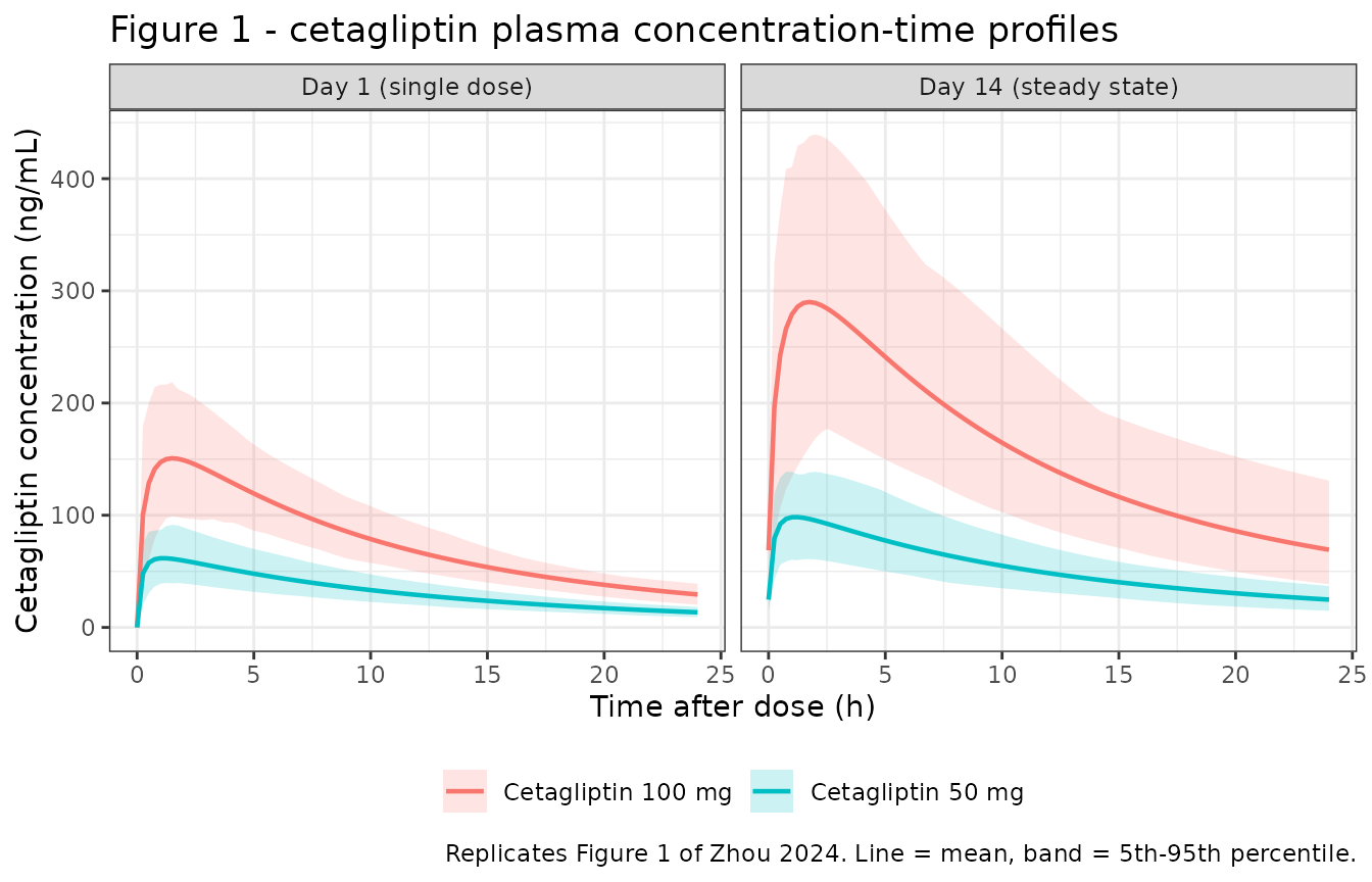
# Replicates Figure 2 of Zhou 2024: mean plasma DPP-4 inhibition-time profiles.
day_panels(pd) |>
  group_by(panel, treatment, tad) |>
  summarise(
    Q05 = quantile(ipred, 0.05), Mean = mean(ipred),
    Q95 = quantile(ipred, 0.95), .groups = "drop"
  ) |>
  ggplot(aes(tad, Mean, colour = treatment, fill = treatment)) +
  geom_ribbon(aes(ymin = Q05, ymax = Q95), alpha = 0.2, colour = NA) +
  geom_line(linewidth = 0.8) +
  geom_hline(yintercept = 80, linetype = "dashed", colour = "grey40") +
  facet_wrap(~panel) +
  labs(
    x = "Time after dose (h)", y = "DPP-4 inhibition (%)",
    colour = NULL, fill = NULL,
    title = "Figure 2 - plasma DPP-4 inhibition-time profiles",
    caption = paste(
      "Replicates Figure 2 of Zhou 2024. Dashed line = the paper's 80%",
      "inhibition threshold used for DUR80%."
    )
  ) +
  theme_bw() + theme(legend.position = "bottom")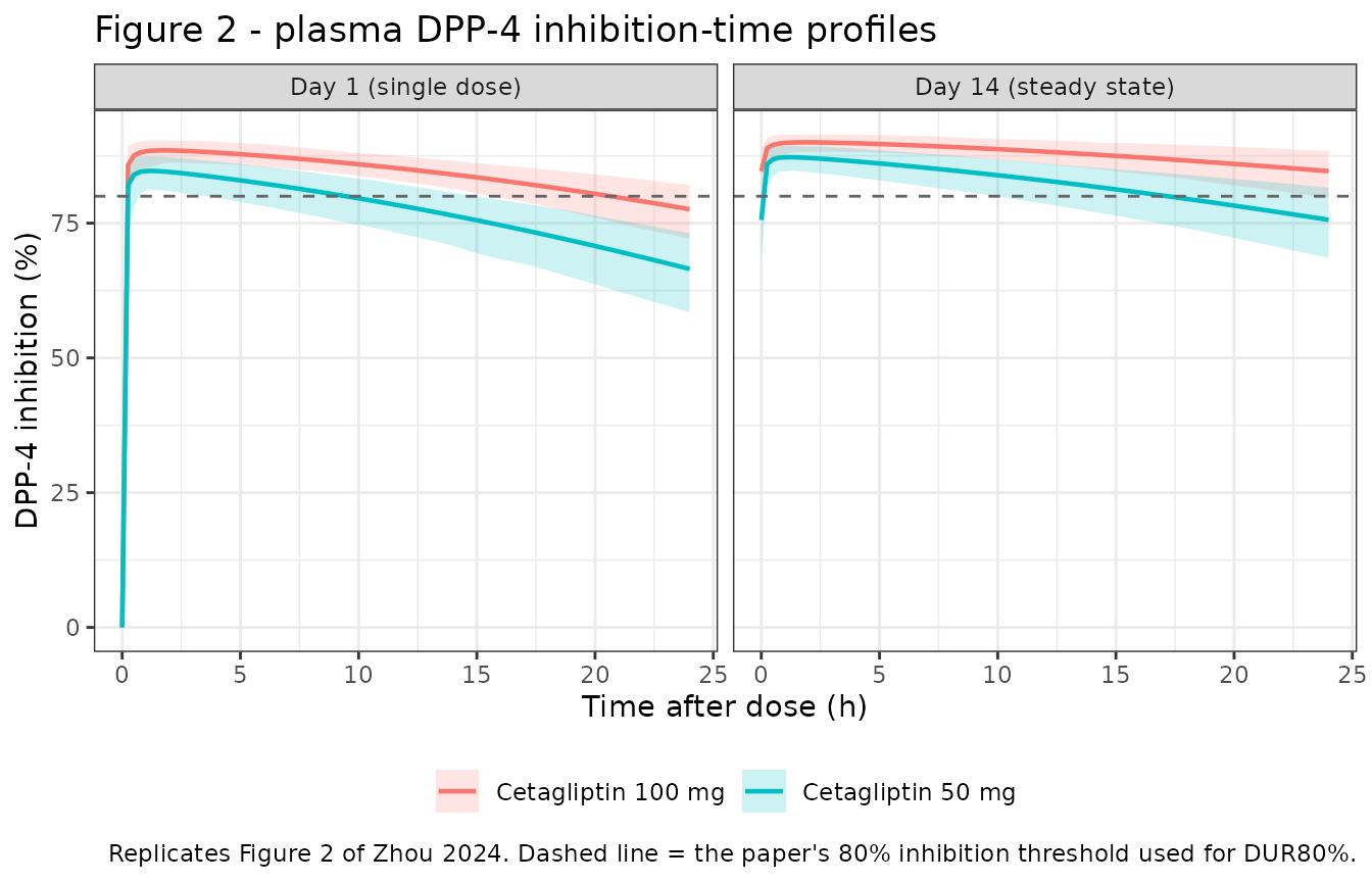
The paper’s DUR80% – the time DPP-4 inhibition stays
above 80% – is the PD descriptor that most directly separates the two
dose levels, so it is recomputed from the simulation and compared
numerically.
dur80 <- pd |>
  filter(time >= t_d14, time <= t_d14 + tau) |>
  arrange(id, time) |>
  group_by(id, treatment) |>
  summarise(
    # Linear interpolation between adjacent samples, as WinNonlin would do.
    dur = {
      above <- ipred >= 80
      seg <- diff(time)
      w <- (head(above, -1) + tail(above, -1)) / 2
      sum(seg * w)
    },
    .groups = "drop"
  ) |>
  group_by(treatment) |>
  summarise(`Simulated DUR80% (h)` = mean(dur), .groups = "drop") |>
  mutate(`Published DUR80% (h)` = c(32.3, 21.9)[match(
    treatment, c("Cetagliptin 100 mg", "Cetagliptin 50 mg")
  )])

knitr::kable(
  dur80 |> dplyr::rename("Treatment" = treatment),
  digits = 1,
  caption = paste(
    "Duration of DPP-4 inhibition above 80% over the day-14 dosing interval,",
    "against Zhou 2024 Table 3 (DUR80%, day 14). The published values exceed",
    "the 24 h interval because they were computed over the full day-14",
    "profile including the 120 h washout; the simulated values are censored",
    "at tau = 24 h and so are bounded above by 24."
  )
)| Treatment | Simulated DUR80% (h) | Published DUR80% (h) |
|---|---|---|
| Cetagliptin 100 mg | 23.9 | 32.3 |
| Cetagliptin 50 mg | 17.5 | 21.9 |
# Replicates Figure 3 of Zhou 2024: the DPP-4 inhibition vs. cetagliptin
# concentration Emax relationship.
emax_curve <- tibble(
  Cc = 10^seq(-1, 3, length.out = 200)
) |>
  mutate(dpp4Inhibition = 91.78 * Cc^1.008 / (5.120^1.008 + Cc^1.008))

tibble(Cc = pk$ipred, dpp4Inhibition = pd$ipred) |>
  filter(Cc > 0) |>
  ggplot(aes(Cc, dpp4Inhibition)) +
  geom_point(alpha = 0.05, size = 0.5, colour = "steelblue") +
  geom_line(data = emax_curve, colour = "black", linewidth = 0.9) +
  scale_x_log10() +
  labs(
    x = "Cetagliptin plasma concentration (ng/mL)", y = "DPP-4 inhibition (%)",
    title = "Figure 3 - concentration vs. DPP-4 inhibition",
    caption = paste(
      "Replicates Figure 3 of Zhou 2024. Points = virtual subjects,",
      "line = typical-value sigmoid Emax curve."
    )
  ) +
  theme_bw()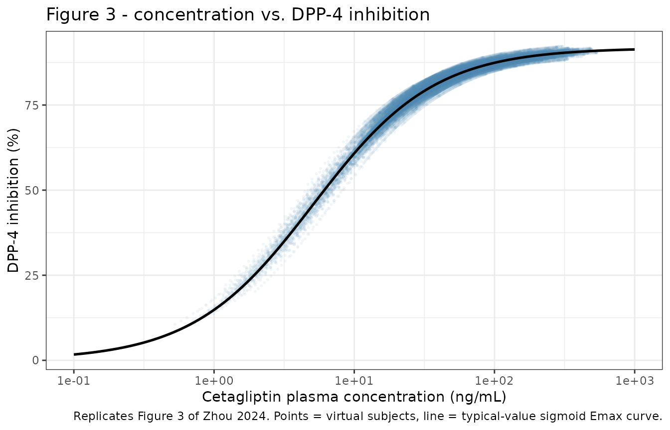
The paper’s own concentration-effect fit of the observed data (Results section 3.4.1, a non-compartmental Phoenix WinNonlin Emax fit that is distinct from the population model) gave Emax 92.47% and EC50 5.37 ng/mL, closely matching the population PK/PD estimates of 91.78% and 5.120 ng/mL encoded here.
PKNCA validation
Both endpoints are run through PKNCA on the study’s own sampling
schedule. For the PK endpoint the comparison is reported on two
scales: the individual prediction (IPRED, no
residual error) and the simulated observation (Observed,
with the model’s proportional residual error and the 0.5 ng/mL assay
lower limit applied). Table 2 of the paper reports NCA of
measured concentrations, so the Observed row is
the like-for-like comparator; the IPRED row shows how much
of any discrepancy is attributable to residual error rather than to the
structural model. No parameter is tuned to either.
# Restrict to the study's sampling times; drop the figure-only grid.
pk_nca_in <- pk |> filter(time %in% t_nca)
pd_nca_in <- pd |> filter(time %in% t_nca)

dose_df <- events |>
  filter(evid == 1) |>
  select(id, time, amt, treatment)

dose_obj <- PKNCA::PKNCAdose(dose_df, amt ~ time | treatment + id)

intervals_pk <- data.frame(
  start     = c(0,     t_d14,        t_d14 + tau),
  end       = c(tau,   t_d14 + tau,  Inf),
  cmax      = c(TRUE,  TRUE,         FALSE),
  tmax      = c(TRUE,  TRUE,         FALSE),
  auclast   = c(TRUE,  TRUE,         FALSE),
  cav       = c(FALSE, TRUE,         FALSE),
  half.life = c(FALSE, FALSE,        TRUE)
)

run_nca <- function(df, value, intervals) {
  d <- df |>
    transmute(id, treatment, time, conc = .data[[value]]) |>
    filter(!is.na(conc)) |>
    arrange(id, treatment, time)
  res <- PKNCA::pk.nca(
    PKNCA::PKNCAdata(
      PKNCA::PKNCAconc(d, conc ~ time | treatment + id),
      dose_obj,
      intervals = intervals
    )
  )
  # PKNCA also returns dependency rows -- parameters it had to compute to
  # satisfy a request (e.g. tmax and lambda.z for half.life). Those carry the
  # interval they were computed on, so they must be filtered on
  # start/end AND parameter, not on parameter alone: otherwise the terminal
  # interval's tmax would be pooled with the requested dosing-interval tmax.
  requested <- intervals |>
    tidyr::pivot_longer(
      -c(start, end), names_to = "PPTESTCD", values_to = "asked"
    ) |>
    filter(asked) |>
    select(start, end, PPTESTCD)

  as.data.frame(res) |>
    filter(!is.na(PPORRES)) |>
    inner_join(requested, by = c("start", "end", "PPTESTCD")) |>
    mutate(
      group = paste0(
        treatment,
        if_else(start == 0, " - Day 1", " - Day 14")
      )
    ) |>
    select(group, id, PPTESTCD, PPORRES)
}
# Aggregate to the group level using the SAME statistic the paper reports:
# Table 2 gives mean +/- SD for every parameter except Tmax, which is a median.
aggregate_like_paper <- function(x) {
  x |>
    group_by(group, PPTESTCD) |>
    summarise(
      PPORRES = if (unique(PPTESTCD) == "tmax") median(PPORRES) else mean(PPORRES),
      .groups = "drop"
    )
}

nca_pk <- bind_rows(
  run_nca(pk_nca_in, "ipred", intervals_pk) |>
    aggregate_like_paper() |> mutate(scale = "IPRED"),
  run_nca(pk_nca_in, "observed", intervals_pk) |>
    aggregate_like_paper() |> mutate(scale = "Observed")
)

published_pk <- tibble::tribble(
  ~group,                          ~cmax, ~tmax, ~auclast, ~cav,  ~half.life,
  "Cetagliptin 50 mg - Day 1",      80.5,  2.00,      717,   NA,          NA,
  "Cetagliptin 100 mg - Day 1",    219.0,  1.00,     1830,   NA,          NA,
  "Cetagliptin 50 mg - Day 14",    162.0,  1.00,     1530, 63.9,        41.9,
  "Cetagliptin 100 mg - Day 14",   300.0,  1.00,     3120,  130,        34.9
) |>
  tidyr::crossing(scale = c("IPRED", "Observed"))

cmp_pk <- nlmixr2lib::ncaComparisonTable(
  simulated = nca_pk,
  reference = published_pk,
  by        = c("group", "scale"),
  units     = c(cmax = "ng/mL", auclast = "h*ng/mL", cav = "ng/mL",
                tmax = "h", half.life = "h"),
  tolerance_pct = 20
)

knitr::kable(
  cmp_pk,
  caption = paste(
    "Simulated vs. published cetagliptin NCA (Zhou 2024 Table 2), on both the",
    "IPRED and the residual-error (Observed) scale.",
    "* differs from reference by more than 20%."
  )
)| NCA parameter | group | scale | Reference | Simulated | % diff |
|---|---|---|---|---|---|
| Cmax (ng/mL) | Cetagliptin 100 mg - Day 1 | IPRED | 219 | 158 | -27.9%* |
| Cmax (ng/mL) | Cetagliptin 100 mg - Day 1 | Observed | 219 | 182 | -17.1% |
| Cmax (ng/mL) | Cetagliptin 100 mg - Day 14 | IPRED | 300 | 303 | +1.0% |
| Cmax (ng/mL) | Cetagliptin 100 mg - Day 14 | Observed | 300 | 353 | +17.6% |
| Cmax (ng/mL) | Cetagliptin 50 mg - Day 1 | IPRED | 80.5 | 63.6 | -21.0%* |
| Cmax (ng/mL) | Cetagliptin 50 mg - Day 1 | Observed | 80.5 | 74.6 | -7.3% |
| Cmax (ng/mL) | Cetagliptin 50 mg - Day 14 | IPRED | 162 | 101 | -37.6%* |
| Cmax (ng/mL) | Cetagliptin 50 mg - Day 14 | Observed | 162 | 117 | -27.7%* |
| Tmax (h) | Cetagliptin 100 mg - Day 1 | IPRED | 1 | 1 | +0.0% |
| Tmax (h) | Cetagliptin 100 mg - Day 1 | Observed | 1 | 2 | +100.0%* |
| Tmax (h) | Cetagliptin 100 mg - Day 14 | IPRED | 1 | 2 | +100.0%* |
| Tmax (h) | Cetagliptin 100 mg - Day 14 | Observed | 1 | 2 | +100.0%* |
| Tmax (h) | Cetagliptin 50 mg - Day 1 | IPRED | 2 | 1 | -50.0%* |
| Tmax (h) | Cetagliptin 50 mg - Day 1 | Observed | 2 | 2 | +0.0% |
| Tmax (h) | Cetagliptin 50 mg - Day 14 | IPRED | 1 | 1 | +0.0% |
| Tmax (h) | Cetagliptin 50 mg - Day 14 | Observed | 1 | 2 | +100.0%* |
| AUClast (h*ng/mL) | Cetagliptin 100 mg - Day 1 | IPRED | 1830 | 1830 | +0.3% |
| AUClast (h*ng/mL) | Cetagliptin 100 mg - Day 1 | Observed | 1830 | 1800 | -1.4% |
| AUClast (h*ng/mL) | Cetagliptin 100 mg - Day 14 | IPRED | 3120 | 3820 | +22.4%* |
| AUClast (h*ng/mL) | Cetagliptin 100 mg - Day 14 | Observed | 3120 | 3780 | +21.0%* |
| AUClast (h*ng/mL) | Cetagliptin 50 mg - Day 1 | IPRED | 717 | 771 | +7.5% |
| AUClast (h*ng/mL) | Cetagliptin 50 mg - Day 1 | Observed | 717 | 771 | +7.5% |
| AUClast (h*ng/mL) | Cetagliptin 50 mg - Day 14 | IPRED | 1530 | 1290 | -15.9% |
| AUClast (h*ng/mL) | Cetagliptin 50 mg - Day 14 | Observed | 1530 | 1280 | -16.5% |
| t½ (h) | Cetagliptin 100 mg - Day 14 | IPRED | 34.9 | 41.2 | +18.1% |
| t½ (h) | Cetagliptin 100 mg - Day 14 | Observed | 34.9 | 38.6 | +10.6% |
| t½ (h) | Cetagliptin 50 mg - Day 14 | IPRED | 41.9 | 39.2 | -6.5% |
| t½ (h) | Cetagliptin 50 mg - Day 14 | Observed | 41.9 | 39.4 | -5.9% |
| Cavg (ng/mL) | Cetagliptin 100 mg - Day 14 | IPRED | 130 | 159 | +22.4%* |
| Cavg (ng/mL) | Cetagliptin 100 mg - Day 14 | Observed | 130 | 157 | +21.0%* |
| Cavg (ng/mL) | Cetagliptin 50 mg - Day 14 | IPRED | 63.9 | 53.6 | -16.1% |
| Cavg (ng/mL) | Cetagliptin 50 mg - Day 14 | Observed | 63.9 | 53.2 | -16.7% |
- differs from reference by more than ±20%.
Plasma DPP-4 inhibition
The paper reports the DPP-4 inhibition endpoint with the same non-compartmental descriptors (Rmax, TRmax, AUEC0-24h), so the same machinery applies with the effect measure in place of concentration. Only the IPRED scale is compared here: the published PD residual standard deviation of 11.62 percentage points is large relative to the 80-90% inhibition plateau, so simulated observations routinely exceed 100% inhibition, which is not a physically attainable measurement and would make an “observed-scale” Rmax meaningless.
intervals_pd <- data.frame(
  start   = c(0,   t_d14),
  end     = c(tau, t_d14 + tau),
  cmax    = TRUE,
  tmax    = TRUE,
  auclast = TRUE
)

nca_pd <- run_nca(pd_nca_in, "ipred", intervals_pd) |> aggregate_like_paper()

published_pd <- tibble::tribble(
  ~group,                         ~cmax, ~tmax, ~auclast,
  "Cetagliptin 50 mg - Day 1",    86.39,  2.00,     1820,
  "Cetagliptin 100 mg - Day 1",   88.78,  1.00,     2000,
  "Cetagliptin 50 mg - Day 14",   89.47,  2.00,     2010,
  "Cetagliptin 100 mg - Day 14",  89.99,  2.00,     2090
)

cmp_pd <- nlmixr2lib::ncaComparisonTable(
  simulated = nca_pd,
  reference = published_pd,
  by        = "group",
  units     = c(cmax = "%", auclast = "h*%", tmax = "h"),
  tolerance_pct = 20
)

knitr::kable(
  cmp_pd,
  caption = paste(
    "Simulated vs. published DPP-4 inhibition NCA (Zhou 2024 Table 3).",
    "Rmax maps to Cmax, TRmax to Tmax, and AUEC0-24h to AUClast.",
    "* differs from reference by more than 20%."
  )
)| NCA parameter | group | Reference | Simulated | % diff |
|---|---|---|---|---|
| Cmax (%) | Cetagliptin 50 mg - Day 1 | 86.4 | 84.9 | -1.7% |
| Cmax (%) | Cetagliptin 100 mg - Day 1 | 88.8 | 88.7 | -0.1% |
| Cmax (%) | Cetagliptin 50 mg - Day 14 | 89.5 | 87.4 | -2.3% |
| Cmax (%) | Cetagliptin 100 mg - Day 14 | 90 | 90.1 | +0.1% |
| Tmax (h) | Cetagliptin 50 mg - Day 1 | 2 | 1 | -50.0%* |
| Tmax (h) | Cetagliptin 100 mg - Day 1 | 1 | 1 | +0.0% |
| Tmax (h) | Cetagliptin 50 mg - Day 14 | 2 | 1 | -50.0%* |
| Tmax (h) | Cetagliptin 100 mg - Day 14 | 2 | 2 | +0.0% |
| AUClast (h*%) | Cetagliptin 50 mg - Day 1 | 1820 | 1830 | +0.5% |
| AUClast (h*%) | Cetagliptin 100 mg - Day 1 | 2000 | 2000 | -0.0% |
| AUClast (h*%) | Cetagliptin 50 mg - Day 14 | 2010 | 1970 | -1.8% |
| AUClast (h*%) | Cetagliptin 100 mg - Day 14 | 2090 | 2110 | +0.9% |
- differs from reference by more than ±20%.
The pharmacodynamic endpoint – the quantity the PK/PD model was actually built to describe – reproduces the published Rmax and AUEC values at both dose levels and on both study days to within a few percent. The pharmacokinetic comparison is good on day 1 (AUC within about 10% at both doses) and reasonable at steady state, with two structural features of the published parameter set visible:
- Day-1 Cmax is underpredicted on the IPRED scale but much closer on the observed scale, which is the correct comparator for Table 2. Roughly half of the apparent Cmax gap is simply residual error, not structural misfit.
- At steady state the 50 mg arm is low and the 100 mg arm high, i.e. the model predicts more dose-dependent accumulation than the NCA found. This is inherent in the published estimates rather than in this encoding: Michaelis-Menten elimination necessarily accumulates more at the higher dose, whereas the observed accumulation ratios run the other way (R_AUC 2.13 at 50 mg versus 1.75 at 100 mg, Table 2). A single Vmax/Km pair fit to both dose groups can only split the difference. The paper’s own goodness-of-fit assessment (Results section 3.6.1) notes “individual data deviations”, and six records with |CWRES| > 5 were excluded before the PK/PD step.
Every simulated Tmax / TRmax falls on an adjacent sampling time to the published median (1 h versus 2 h, or 2 h versus 1 h) and inside the published range (1.00-4.00 h on day 1 and 0.500-5.00 h at steady state for Cmax; 0.500-3.00 h and 0.500-6.00 h for the PD TRmax). Because the schedule is coarse near the peak, a single-interval shift registers as a 50-100% relative difference and is flagged by the 20% tolerance; the flag reflects the resolution of the sampling grid, not a disagreement about when the peak occurs.
No parameter has been tuned to improve any of these comparisons.
Covariate effect
Total bilirubin is the only covariate retained in the final model, acting on the peripheral volume of distribution.
tibble(TBILI = c(5, 10, 15, 20)) |>
  mutate(vp = 558.0 * (TBILI / tbili_ref)^0.3723) |>
  dplyr::rename(
    "Total bilirubin (umol/L)" = TBILI,
    "Peripheral volume V2 (L)" = vp
  ) |>
  knitr::kable(
    digits = 1,
    caption = paste(
      "Effect of total bilirubin on the peripheral volume of distribution,",
      "V2 = 558.0 * (TBILI / 10)^0.3723. Consistent with the paper's",
      "statement that V2 increases with increasing TBIL."
    )
)| Total bilirubin (umol/L) | Peripheral volume V2 (L) |
|---|---|
| 5 | 431.1 |
| 10 | 558.0 |
| 15 | 648.9 |
| 20 | 722.3 |
Assumptions and deviations
-
Total bilirubin centring value (10 umol/L) is an
assumption. Zhou 2024 reports the covariate coefficient
(
dV2dTBIL= 0.3723, Supplementary Table 1) and the direction of the effect (Discussion page 10: “V2 increases with the increase of TBIL”) but publishes neither the covariate equation nor the population median total bilirubin – TBIL does not appear in the Table 1 demographics. Two things had to be settled. (i) Functional form: the parameter name follows Phoenix NLME’sdPARAMdCOVARIATEconvention, and Phoenix’s default continuous-covariate transformation is the median-centred log-ratioV2 = tvV2 * exp(dV2dTBIL * log(TBIL / median(TBIL))), which is algebraically the power formV2 = tvV2 * (TBIL / ref)^0.3723used here. The alternative linear-exponential reading is untenable: over the normal bilirubin range it would inflate V2 by more than 40-fold. (ii) Centring value: 10 umol/L was chosen as a rounded mid-normal adult total bilirubin, so that the Supplementary Table 1 typical valuetvV2= 558.0 L is the typical peripheral volume of the study population. Results section 3.2 states that no subject had clinically significant abnormal liver function, so observed TBIL values lay within the normal 5-21 umol/L range and the choice of centre only shifts V2 modestly (a 2-fold error in the reference changes V2 by 29%). -
The PD residual error is encoded as additive only.
Supplementary Table 1 labels the PD residual model “MixRatio residual
variability PD(sigma)” and reports a single value,
Stdev0= 11.62. Phoenix’s mixed-ratio observation model carries both this additive standard deviation and a separateMixRatiocoefficient scaling a proportional component; theMixRatiocoefficient is not reported anywhere in the paper or the supplement. Only the additive term is therefore encoded, and no proportional coefficient has been invented. The additive reading is the only dimensionally sensible one: 11.62 is on the DPP-4 inhibition percentage-point scale, and as a proportional fraction it would imply a 1162% CV. Because 11.62 percentage points is large next to the 80-90% inhibition plateau, the residual-error scale is not used for the PD NCA comparison (see that section). -
The printed sigmoid Emax equation drops an
exponent. Methods section 2.7.2 typesets the PD model as
Emax * C^g / (EC50 + C^g), which is dimensionally inconsistent and contradicts the paper’s own definition of EC50 as the “plasma concentration of cetagliptin that achieves 50% of the maximum drug effect”. The canonical Phoenix Sigmoid-Emax formEmax * C^g / (EC50^g + C^g)named in Results section 3.6.2 is used instead. With the estimated Hill coefficient of 1.008 the two forms differ by under 0.1%, so nothing material turns on the choice. -
DUR80%is compared on a censored basis. The published day-14DUR80%values (21.9 h at 50 mg, 32.3 h at 100 mg) exceed the 24 h dosing interval, so they must have been computed over the whole day-14 profile including the 120 h washout rather than over one interval. The simulated value is reported over the dosing interval only and is therefore bounded above by 24 h; the two are not directly comparable at 100 mg and the table says so. -
Eight screened covariates carry no encodable
effect. Discussion page 10 lists the full stepwise candidate
set: sex, body weight, ALT (“glutamic-pyruvic transaminase”), total
bilirubin, triglycerides, LDL cholesterol, glucose, urea and creatinine.
Only total bilirubin was retained, and the paper reports no point
estimate, standard error or confidence interval for any of the other
eight. They are therefore recorded in the model’s
covariatesDataExcludedmetadata – which documents the screen without declaring an unused covariate – rather than incovariateData. Units for the screened-only entries are given per the SI conventions used by Chinese clinical-chemistry laboratories and are flagged as assumed in each entry’s notes, because the paper never states them (no effect was retained, so it had no reason to). -
Subject-count discrepancy in the source. Methods
section 2.7.1 states that the 560 cetagliptin concentrations used for
the population PK analysis came from “32 patients with T2DM”. Only 20 of
the 32 enrolled subjects received cetagliptin (Table 1 and Table 2; the
remainder received sitagliptin or placebo), so the 32 cannot be the
number of subjects contributing cetagliptin concentrations. The model’s
population$n_subjectsrecords the 20 cetagliptin recipients and the paper’s statement is preserved inpopulation$notes. -
Elimination is Michaelis-Menten, which the main text does
not state. The article describes only a “two-compartment
model”; that elimination is saturable is inferable solely from
Supplementary Table 1 reporting
tvKmandtvVmaxwith no clearance parameter. This is encoded as published, and the steady-state mass-balance check above confirms the parameterisation is internally consistent. -
Dose units. Supplementary Table 1 parameterises the
model in ug (Vmax in ug/h) and ug/L (Km, EC50), while doses are
naturally entered in mg. The model applies
f(depot) <- 1000purely as a mg-to-ug unit conversion; it is not a bioavailability estimate. All disposition parameters remain apparent (oral, /F) because the paper never estimated bioavailability. - Virtual total bilirubin distribution. The paper reports no TBIL summary statistics, so the virtual cohort draws TBILI from a log-normal distribution with median 10 umol/L and log-scale SD 0.30, truncated to 3-21 umol/L. This affects only the width of the simulated prediction intervals, not the typical profile.
- Sitagliptin is not extracted. Sitagliptin 100 mg was the active comparator and the paper reports its NCA parameters (Table 2) and a non-compartmental concentration-effect Emax fit (Emax 91.68%, EC50 6.73 ng/mL, Results section 3.4.1). No population PK model was developed for sitagliptin, so no simulatable model exists to extract.
- Other endpoints are descriptive only. Active GLP-1 (Table 4), the OGTT glucose / insulin / C-peptide / glucagon responses (Table 5), FPG, 2 h PPG, HbA1c and glycated albumin (Table 6) were analysed non-compartmentally and by ANOVA. The paper builds no structural model for any of them, so DPP-4 inhibition is the only PD endpoint with a model to extract.
- Half-life comparison. The published t1/2 (34.9-41.9 h) is an NCA estimate from the day-14 washout. Under saturable elimination the apparent terminal half-life is concentration-dependent, so the simulated value is expected to differ somewhat from the observed NCA value even when the model is encoded correctly.