Ceftriaxone (Tsai 2023)
Source:vignettes/articles/Tsai_2023_ceftriaxone.Rmd
Tsai_2023_ceftriaxone.RmdModel and source
- Citation: Tsai D, Zam BB, Tongs C, Chiong F, Sajiv C, Pawar B, Ashok A, Cooper BP, Tong SYC, Janson S, Wallis SC, Roberts JA, Parker SL. Validating a novel three-times-weekly post-hemodialysis ceftriaxone regimen in infected Indigenous Australian patients-a population pharmacokinetic study. J Antimicrob Chemother. 2023;78(8):1963-1973. doi:10.1093/jac/dkad190.
- Article: https://doi.org/10.1093/jac/dkad190
- Supplement (Tables S1-S3, Figure S1): https://doi.org/10.1093/jac/dkad190 (JAC Online supplementary data)
Tsai and colleagues studied a novel 2 g three-times-weekly post-dialysis ceftriaxone regimen in Indigenous Australian adults with end-stage renal disease. The regimen is designed to align every ceftriaxone dose with an existing dialysis session so that no additional venous cannulation is needed – vein preservation matters greatly in a population that may require hemodialysis for decades.
The model has three features that make it unusual for a beta-lactam popPK model, and all three are reproduced here:
-
Explicit albumin binding. Rather than assuming a
fixed unbound fraction, the model carries protein-bound ceftriaxone as
its own state and exchanges it with unbound drug through second-order
association (
k1) and first-order dissociation (k2) rate constants. Both total and unbound plasma concentrations are model outputs. This matters because the measured unbound fraction in this cohort (median 0.29) was far higher than in healthy individuals (0.04-0.17). -
Dialysis replaces, rather than augments, clearance.
The Table S2 model file states
IF (HDx.EQ.1) CL = CL_HD, so while a session runs the interdialytic clearance arm is switched out entirely for a > 10-fold larger dialytic clearance. This differs from the additive dialysis-arm convention used elsewhere innlmixr2lib(Veinstein_2013_gentamicin,Eyler_2014_ertapenem,Jacobs_2016_colistin). - Bilirubin, not creatinine, drives clearance. In anuric patients the biliary route dominates, so clearance falls with serum bilirubin through an inverse-power relationship.
Population
Sixteen Indigenous Australian adults (13 female, 81%) on three-times-weekly intermittent high-flux hemodialysis contributed 122 plasma samples assayed for both total and unbound ceftriaxone (Tsai 2023 Table 1). Median age was 57 years (IQR 51-64) and median weight 71 kg (IQR 59-83). Median serum albumin was 36 g/L (IQR 33-39) and median total bilirubin 10 umol/L (IQR 6-14); seven subjects had bilirubin above 10 umol/L, all of acute cause (two cholecystitis, five severe infection). Infection sources were respiratory (11), urinary (1), bacteremia (1), skin and soft tissue (1) and intra-abdominal (1). Dialyzers were high-flux throughout: FX80 (3), FX100 (10), FX120 (3).
The same information is available programmatically via
readModelDb("Tsai_2023_ceftriaxone")()$population.
pop <- readModelDb("Tsai_2023_ceftriaxone")()$population
str(pop[c("species", "n_subjects", "n_samples", "age_median", "weight_median")])
#> List of 5
#>  $ species      : chr "human"
#>  $ n_subjects   : int 16
#>  $ n_samples    : int 122
#>  $ age_median   : chr "57 years (IQR 51-64); full range not reported"
#>  $ weight_median: chr "71 kg (IQR 59-83); full range not reported"
Source trace
Every ini() entry carries an in-file comment naming its
source location. The table below collects them for review. “Table S2”
refers to the Pmetrics model file reproduced in the supplementary
data.
| Equation / parameter | Value | Source location |
|---|---|---|
lcl (CLnHD) |
0.83 L/h | Table 2, Mean column (SD 0.28, CV 33.33%, median 0.77) |
lcl_hemodialysis (CLHD) |
8.76 L/h | Table 2, Mean column (SD 1.85, CV 21.10%, median 9.13) |
lvc (Vc) |
2.25 L | Table 2, Mean column (SD 1.71, CV 75.81%, median 1.91) |
lk1 (Kon) |
1.18 L/mg/h | Table 2, Mean column (SD 0.33, CV 27.76%, median 1.18) |
lk2 (Koff) |
206.37 1/h | Table 2, Mean column (SD 48.38, CV 23.44%, median 202.36) |
lk12 (Kcp) |
15.37 1/h | Table 2, Mean column (SD 7.24, CV 47.10%, median 17.01) |
lk21 (Kpc) |
0.78 1/h | Table 2, Mean column (SD 0.50, CV 64.05%, median 0.55) |
e_tbili_cl |
0.5 (fixed) | Table S2 secondary variables:
CL=CL_nHD*(14.1/Bili)**0.5; same form in Results |
| bilirubin reference 14.1 umol/L | constant | Table S2 secondary variables (hard-coded; derivation not stated) |
bmax_per_g_alb = 16.7 mg/g |
constant | Table S2 secondary variables: Bmax1=Alb*Vc*16.7
|
All seven eta variances |
omega^2 = log(CV^2+1) | Table 2, CV% column (see Assumptions) |
addSd, addSd_Cunbound
|
0.3 mg/L | Table S2 #Error block, C0 for both outputs |
propSd, propSd_Cunbound
|
0.1 | Table S2 #Error block, C1 for both outputs |
d/dt(central), d/dt(complex),
d/dt(peripheral1)
|
n/a | Table S2 #Differential equations (XP(1), XP(2),
XP(3)) |
Cunbound, Cc
|
n/a | Table S2 #Output equations (Y(1), Y(2)) |
| Dialysis switch | n/a | Table S2 secondary variables:
&IF (HDx.EQ.1) CL=CL_HD
|
| Compartment diagram | n/a | Figure S1 |
The 16.7 mg ceftriaxone bound per gram of albumin
encodes 2 binding sites per albumin molecule, which is
a useful independent check on the transcription:
# 2 sites * MW(ceftriaxone) / MW(albumin) * 1000 mg/g
2 * 554.58 / 66437 * 1000
#> [1] 16.69491
Model structure
mod <- readModelDb("Tsai_2023_ceftriaxone")
mod
#> function() {
#>   description <- "Two-compartment population PK model for intravenous ceftriaxone in Indigenous Australian adults with end-stage renal disease on three-times-weekly intermittent high-flux hemodialysis, receiving a novel 2 g three-times-weekly post-dialysis regimen. PK is parameterised on unbound drug: the central state carries unbound ceftriaxone and an explicit second-order albumin-binding exchange (k1 on / k2 off) against a capacity bmax derived from serum albumin carries the bound drug, so total and unbound plasma concentrations are both model outputs. Clearance is replaced (not augmented) by a > 10-fold higher dialytic clearance while a session is running, gated by the time-varying RRT_HEMODIAL_ACTIVE covariate; interdialytic clearance falls with serum bilirubin through an inverse-power relationship. Estimated with the Pmetrics non-parametric adaptive grid (NPAG). Tsai 2023, n = 16 subjects, 122 total-and-unbound plasma samples."
#>   reference <- paste(
#>     "Tsai D, Zam BB, Tongs C, Chiong F, Sajiv C, Pawar B, Ashok A, Cooper BP,",
#>     "Tong SYC, Janson S, Wallis SC, Roberts JA, Parker SL. Validating a novel",
#>     "three-times-weekly post-hemodialysis ceftriaxone regimen in infected",
#>     "Indigenous Australian patients-a population pharmacokinetic study. J",
#>     "Antimicrob Chemother. 2023;78(8):1963-1973. doi:10.1093/jac/dkad190.",
#>     sep = " "
#>   )
#>   vignette <- "Tsai_2023_ceftriaxone"
#>   units <- list(time = "h", dosing = "mg", concentration = "mg/L")
#>
#>   # Issue #482: what each ODE state holds, in what amount units, in what
#>   # biological matrix. analyte/specimen proposed by a local model from the
#>   # model description; units derived from the units block. verified = FALSE
#>   # means NOT checked against the source paper.
#>   compartmentData <- list(
#>     central = list(analyte = "unbound ceftriaxone", units = "mg", specimen = "plasma", verified = FALSE),
#>     complex = list(analyte = "bound ceftriaxone", units = "mg", specimen = "serum", verified = FALSE),
#>     peripheral1 = list(analyte = "ceftriaxone", units = "mg", specimen = "plasma", verified = FALSE)
#>   )
#>
#>   covariateData <- list(
#>     TBILI = list(
#>       description = "Total serum bilirubin concentration",
#>       units = "umol/L",
#>       type = "continuous",
#>       reference_category = NULL,
#>       notes = "Time-fixed per subject in the source analysis. The only covariate retained in the final model (Tsai 2023 Results, 'Population pharmacokinetic model and model diagnostics': serum bilirubin was 'the only covariate retained in the final model'). Enters as an inverse-power effect on the interdialytic clearance arm, CL = CLnHD * (14.1 / bili)^0.5 (Tsai 2023 Results equation 'When dialysis is off', reproduced verbatim as 'CL=CL_nHD*(14.1/Bili)**0.5' in the Table S2 Pmetrics model file). Clearance and bilirubin followed an inverse-power relationship with r^2 = 0.74 (Figure 2); with the single highest-bilirubin subject (72 umol/L) removed, r^2 = 0.70. Cohort median 10 umol/L (IQR 6-14); 7 of 16 subjects had bilirubin > 10 umol/L, all acute (2 cholecystitis, 5 severe infection). Must be strictly positive: the covariate enters as a denominator, so TBILI = 0 is undefined. The 14.1 umol/L reference value is hard-coded in the Table S2 model file and the paper does not state its derivation (it is not the cohort median of 10 umol/L); it is carried here exactly as printed.",
#>       source_name = "Bili"
#>     ),
#>     ALB = list(
#>       description = "Serum albumin concentration",
#>       units = "g/L",
#>       type = "continuous",
#>       reference_category = NULL,
#>       notes = "Time-fixed per subject in the source analysis. Not a covariate on any structural PK parameter; instead it sets the albumin-binding capacity of the central compartment through the Table S2 secondary variable Bmax1 = Alb * Vc * 16.7 (mg). The 16.7 mg ceftriaxone per g albumin constant encodes 2 binding sites per albumin molecule: 2 * 554.58 (ceftriaxone g/mol) / 66437 (albumin g/mol) * 1000 mg/g = 16.7, consistent with the paper's complex-binding definition (Methods: 'N is the number of ceftriaxone-binding sites per albumin molecule'). Cohort median 36 g/L (IQR 33-39); only one subject had albumin < 30 g/L (at 28 g/L), which the Discussion cites as the reason serum albumin had limited independent influence on the PK model.",
#>       source_name = "Alb"
#>     ),
#>     RRT_HEMODIAL_ACTIVE = list(
#>       description = "Hemodialysis-active indicator (1 while an intermittent high-flux hemodialysis session is running, 0 in the interdialytic interval)",
#>       units = "(binary)",
#>       type = "binary",
#>       reference_category = "0 (no dialysis session running)",
#>       notes = "Time-varying within subject. Implemented in the source as the Pmetrics conditional 'IF (HDx.EQ.1) CL = CL_HD' (Table S2 secondary variables), i.e. the dialytic clearance REPLACES the interdialytic clearance arm for the duration of the session rather than being added to it. This is the opposite composition rule from the additive dialysis-arm precedents (Veinstein 2013 gentamicin, Eyler 2014 ertapenem, Jacobs 2016 colistin); it is encoded here as the paper wrote it. Because CL_HD replaces CL entirely, the bilirubin covariate does not act during a dialysis session. Ceftriaxone clearance was > 10-fold higher during dialysis (8.76 vs 0.83 L/h), which the authors attribute to the high-flux membranes used (FX80 / FX100 / FX120, Fresenius); prior studies using low-flux dialyzers reported no dialytic enhancement. Doses in this study were given post-dialysis (within 5 min of the end of the session), so RRT_HEMODIAL_ACTIVE = 0 at the dosing times of the observed data; it is set to 1 only to reproduce the paper's counterfactual 'administered during dialysis' simulation.",
#>       source_name = "HDx"
#>     )
#>   )
#>
#>   population <- list(
#>     species = "human",
#>     n_subjects = 16L,
#>     n_studies = 1L,
#>     n_samples = 122L,
#>     age_median = "57 years (IQR 51-64); full range not reported",
#>     weight_median = "71 kg (IQR 59-83); full range not reported",
#>     sex_female_pct = 81.25,
#>     race_ethnicity = "100% Indigenous Australian (an explicit inclusion criterion, identified by electronic health record). The Discussion notes that inter-ethnic PK differences are considered unlikely for ceftriaxone, so the authors regard the estimates as transferable to other ethnic origins.",
#>     disease_state = "Adults with end-stage renal disease established on three-times-weekly intermittent hemodialysis, treated with ceftriaxone for an active infection. Sources of infection: respiratory 11, urinary 1, bacteremia 1, skin and soft tissue 1, intra-abdominal 1. Baseline laboratory values (median, IQR): albumin 36 g/L (33-39), urea 15.1 mmol/L (12.2-19.2), total bilirubin 10 umol/L (6-14), ALP 216 U/L (171-338), GGT 74 U/L (42-133), ALT 23 U/L (13-29). Seven subjects had bilirubin > 10 umol/L, all of acute cause.",
#>     renal_function = "Anuric / end-stage renal disease requiring intermittent hemodialysis three times weekly. Exact renal function was not quantifiable because serum creatinine depended on time since the last dialysis session (stated study limitation). Dialyzers were high-flux: FX80 in 3 subjects (19%), FX100 in 10 (63%), FX120 in 3 (19%) (Fresenius Medical Care).",
#>     dose_range = "2 g ceftriaxone (Ceftriaxone-AFT) dissolved in 10 mL water-for-injection, slowly injected into the fistula or central venous cannula within 5 min after the conclusion of each dialysis session, three times weekly.",
#>     regions = "Australia (renal dialysis unit of a remote Northern Territory primary referral centre, Alice Springs Hospital)",
#>     protein_binding = "Measured directly rather than assumed: median unbound fraction 0.29 (IQR 0.20-0.40), substantially higher than the 0.04-0.17 reported for healthy individuals. Median pre-dialysis unbound trough was 18.2 mg/L (IQR 9.7-25.9) over a 2-day interval and 8.8 mg/L (IQR 7.1-17.7) over a 3-day interval; unbound concentrations fell by a median 70% (IQR 64-74%) across each dialysis session.",
#>     notes = "Prospective population PK study. Plasma sampled over two dosing intervals: immediately before and after dialysis, then 5, 15, 60 and 1440 min after the dose, then at 2880 min (or immediately before the next dialysis session for a 48 h interval), and immediately before the next session for a 72 h interval. Total and unbound ceftriaxone assayed by validated UPLC-MS/MS (Table S1); unbound fraction isolated by ultracentrifugation at 37 C with Centrifree devices. One sample was below LLOQ (drawn before any ceftriaxone was given) and was carried into the analysis as 0.0 mg/L. Exclusion criterion: pregnancy."
#>   )
#>
#>   ini({
#>     # Structural parameters: Tsai 2023 Table 2, 'Mean' column of the
#>     # Pmetrics NPAG non-parametric population distribution. Table 2 also
#>     # reports a 'Median' column; the mean is used as the typical value
#>     # here and the median is noted per line. Only the seven primary
#>     # variables of the Table S2 model file are estimated; Vd and the two
#>     # half-lives in Table 2 are flagged there as manually calculated
#>     # derived quantities and are not model parameters.
#>     lcl <- log(0.83)
#>     label("Interdialytic (dialysis-off) clearance CLnHD (L/h)")
#>     # Tsai 2023 Table 2: CLnHD mean 0.83, SD 0.28, CV 33.33%, median 0.77 L/h
#>
#>     lcl_hemodialysis <- log(8.76)
#>     label("Intradialytic (dialysis-on) clearance CLHD (L/h)")
#>     # Tsai 2023 Table 2: CLHD mean 8.76, SD 1.85, CV 21.10%, median 9.13 L/h
#>
#>     lvc <- log(2.25)
#>     label("Central volume of distribution Vc (L)")
#>     # Tsai 2023 Table 2: Vc mean 2.25, SD 1.71, CV 75.81%, median 1.91 L
#>
#>     lk1 <- log(1.18)
#>     label("Second-order ceftriaxone-albumin association rate constant Kon (L/mg/h)")
#>     # Tsai 2023 Table 2: Kon mean 1.18, SD 0.33, CV 27.76%, median 1.18 L/mg/h
#>
#>     lk2 <- log(206.37)
#>     label("First-order ceftriaxone-albumin dissociation rate constant Koff (1/h)")
#>     # Tsai 2023 Table 2: Koff mean 206.37, SD 48.38, CV 23.44%, median 202.36 1/h
#>
#>     lk12 <- log(15.37)
#>     label("Central-to-peripheral rate constant Kcp (1/h)")
#>     # Tsai 2023 Table 2: Kcp mean 15.37, SD 7.24, CV 47.10%, median 17.01 1/h
#>
#>     lk21 <- log(0.78)
#>     label("Peripheral-to-central rate constant Kpc (1/h)")
#>     # Tsai 2023 Table 2: Kpc mean 0.78, SD 0.50, CV 64.05%, median 0.55 1/h
#>
#>     # Bilirubin effect on the interdialytic clearance arm. The exponent is
#>     # hard-coded in the Table S2 model file rather than reported as an
#>     # estimated THETA in Table 2, so it is encoded as fixed().
#>     e_tbili_cl <- fixed(0.5)
#>     label("Inverse-power exponent of total bilirubin on interdialytic CL (unitless)")
#>     # Tsai 2023 Table S2 secondary variables: CL=CL_nHD*(14.1/Bili)**0.5;
#>     # same form printed in Results ('When dialysis is off'). Equivalent to
#>     # (TBILI / 14.1)^-0.5. Supported by the Figure 2 inverse-power fit
#>     # (r^2 = 0.74; r^2 = 0.70 excluding the 72 umol/L subject).
#>
#>     # Interindividual variability. Pmetrics NPAG estimates a discrete
#>     # non-parametric distribution rather than a parametric omega matrix;
#>     # Table 2 summarises that distribution by its mean, SD and CV%. The
#>     # CV% is carried here into a log-normal random effect using the
#>     # standard omega^2 = log(CV^2 + 1) identity. This is a parametric
#>     # APPROXIMATION of a non-parametric distribution (see vignette
#>     # 'Assumptions and deviations'); it is required to reproduce the
#>     # paper's own Monte Carlo PTA simulations, which sample the
#>     # population distribution.
#>     #   CLnHD : 33.33% CV -> omega^2 = log(0.3333^2 + 1) = 0.105341
#>     #   CLHD  : 21.10% CV -> omega^2 = log(0.2110^2 + 1) = 0.043558
#>     #   Vc    : 75.81% CV -> omega^2 = log(0.7581^2 + 1) = 0.454075
#>     #   Kon   : 27.76% CV -> omega^2 = log(0.2776^2 + 1) = 0.074237
#>     #   Koff  : 23.44% CV -> omega^2 = log(0.2344^2 + 1) = 0.053487
#>     #   Kcp   : 47.10% CV -> omega^2 = log(0.4710^2 + 1) = 0.200359
#>     #   Kpc   : 64.05% CV -> omega^2 = log(0.6405^2 + 1) = 0.343760
#>     etalcl              ~ 0.105341  # Tsai 2023 Table 2 (CLnHD, CV 33.33%)
#>     etalcl_hemodialysis ~ 0.043558  # Tsai 2023 Table 2 (CLHD,  CV 21.10%)
#>     etalvc              ~ 0.454075  # Tsai 2023 Table 2 (Vc,    CV 75.81%)
#>     etalk1              ~ 0.074237  # Tsai 2023 Table 2 (Kon,   CV 27.76%)
#>     etalk2              ~ 0.053487  # Tsai 2023 Table 2 (Koff,  CV 23.44%)
#>     etalk12             ~ 0.200359  # Tsai 2023 Table 2 (Kcp,   CV 47.10%)
#>     etalk21             ~ 0.343760  # Tsai 2023 Table 2 (Kpc,   CV 64.05%)
#>
#>     # Residual error. Table S2 '#Error' block gives one assay-error
#>     # polynomial per output equation, identical for both:
#>     #   0.3, 0.1, 0, 0   ->  SD = 0.3 + 0.1 * conc  (C2 = C3 = 0)
#>     # so each output carries a 0.3 mg/L additive plus 10% proportional
#>     # term. The C1 = 0.1 slope is consistent with the Table S1 assay
#>     # validation (precision within 8.4% total, 7.5% unbound).
#>     # NOTE: Pmetrics multiplies this assay polynomial by an estimated
#>     # noise-inflation factor gamma; the Table S2 file sets the gamma
#>     # STARTING value 'G=2', and the paper does not report the final
#>     # estimated gamma anywhere. The assay polynomial is therefore carried
#>     # here unscaled (equivalent to gamma = 1), which is the minimum-
#>     # assumption reading of the published Table S2 file. See vignette 'Assumptions
#>     # and deviations'.
#>     addSd <- 0.3
#>     label("Additive residual error on total Cc (mg/L)")
#>     # Tsai 2023 Table S2 #Error, output 2 (total): C0 = 0.3
#>     propSd <- 0.1
#>     label("Proportional residual error on total Cc (fraction)")
#>     # Tsai 2023 Table S2 #Error, output 2 (total): C1 = 0.1
#>     addSd_Cunbound <- 0.3
#>     label("Additive residual error on unbound Cunbound (mg/L)")
#>     # Tsai 2023 Table S2 #Error, output 1 (unbound): C0 = 0.3
#>     propSd_Cunbound <- 0.1
#>     label("Proportional residual error on unbound Cunbound (fraction)")
#>     # Tsai 2023 Table S2 #Error, output 1 (unbound): C1 = 0.1
#>   })
#>
#>   model({
#>     # Stoichiometric constant for the albumin-binding capacity, carried
#>     # exactly as hard-coded in the Table S2 secondary variable
#>     # Bmax1 = Alb * Vc * 16.7. Units: mg ceftriaxone bound per g albumin.
#>     # It encodes 2 binding sites per albumin molecule --
#>     #   2 * 554.58 (ceftriaxone g/mol) / 66437 (albumin g/mol) * 1000 = 16.7
#>     # -- matching the paper's complex-binding definition (Methods: Bmax is
#>     # a function of N binding sites, MCTX and MAlb).
#>     bmax_per_g_alb <- 16.7
#>
#>     # Reference bilirubin for the inverse-power clearance covariate
#>     # (umol/L). Hard-coded in the Table S2 model file; the paper does not
#>     # state its derivation.
#>     tbili_ref <- 14.1
#>
#>     # Individual parameters.
#>     cl              <- exp(lcl + etalcl) * (tbili_ref / TBILI)^e_tbili_cl
#>     cl_hemodialysis <- exp(lcl_hemodialysis + etalcl_hemodialysis)
#>     vc              <- exp(lvc + etalvc)
#>     k1              <- exp(lk1 + etalk1)
#>     k2              <- exp(lk2 + etalk2)
#>     k12             <- exp(lk12 + etalk12)
#>     k21             <- exp(lk21 + etalk21)
#>
#>     # Dialysis REPLACES the interdialytic clearance arm rather than adding
#>     # to it (Table S2: 'IF (HDx.EQ.1) CL = CL_HD'). Note this differs from
#>     # the additive dialysis-arm convention used by Veinstein 2013 /
#>     # Eyler 2014 / Jacobs 2016; it is encoded as Tsai 2023 wrote it.
#>     cl_total <- (1 - RRT_HEMODIAL_ACTIVE) * cl + RRT_HEMODIAL_ACTIVE * cl_hemodialysis
#>     kel      <- cl_total / vc
#>
#>     # Albumin-binding capacity of the central compartment, as a MASS (mg)
#>     # rather than a concentration -- so it is directly comparable with the
#>     # bound-drug amount held in the 'complex' state (Table S2).
#>     bmax <- ALB * vc * bmax_per_g_alb
#>
#>     # ODE system, transcribed from the Table S2 '#Differential equations'
#>     # block. X(1) -> central (unbound drug), X(2) -> complex (albumin-bound
#>     # drug), X(3) -> peripheral1. Elimination and inter-compartmental
#>     # distribution act on unbound drug only; the bound state exchanges
#>     # solely with central.
#>     #   XP(1) = RATEIV(1) - (Ke + Kcp)*X(1) - (Kon/Vc)*(Bmax1-X(2))*X(1)
#>     #                     + Koff*X(2) + Kpc*X(3)
#>     #   XP(2) =             (Kon/Vc)*(Bmax1-X(2))*X(1) - Koff*X(2)
#>     #   XP(3) =  Kcp*X(1) - Kpc*X(3)
#>     # The dose enters 'central' (Pmetrics RATEIV(1)) via the event table.
#>     d/dt(central) <- -(kel + k12) * central -
#>       (k1 / vc) * (bmax - complex) * central + k2 * complex + k21 * peripheral1
#>     d/dt(complex) <-
#>       (k1 / vc) * (bmax - complex) * central - k2 * complex
#>     d/dt(peripheral1) <- k12 * central - k21 * peripheral1
#>
#>     # Output equations (Table S2 '#Output equations').
#>     #   Y(1) = X(1)/Vc          -> unbound plasma concentration
#>     #   Y(2) = (X(2)+X(1))/Vc   -> total plasma concentration
#>     Cunbound <- central / vc
#>     Cc       <- (complex + central) / vc
#>
#>     Cc       ~ add(addSd) + prop(propSd)
#>     Cunbound ~ add(addSd_Cunbound) + prop(propSd_Cunbound)
#>   })
#> }
#> <environment: 0x55679fb0cd78>
Virtual cohort
Original observed data are not publicly available. The cohort below reproduces the Table 1 covariate distributions: serum albumin centred on the observed median of 36 g/L and total bilirubin log-normally distributed with median 10 umol/L and an IQR close to the observed 6-14 umol/L.
set.seed(20230801)
n_sub <- 200L  # 200 per arm is the vignette cap

cohort <- tibble(
  id    = seq_len(n_sub),
  TBILI = pmax(1, rlnorm(n_sub, meanlog = log(10), sdlog = 0.55)),
  ALB   = pmax(20, rnorm(n_sub, mean = 36, sd = 5))
)

quantile(cohort$TBILI, c(0.25, 0.5, 0.75))  # paper: 10 (IQR 6-14) umol/L
#>      25%      50%      75%
#>  7.26600 10.19930 15.40894
quantile(cohort$ALB,   c(0.25, 0.5, 0.75))  # paper: 36 (IQR 33-39) g/L
#>      25%      50%      75%
#> 32.69399 35.81122 39.99856
A helper builds event tables. Two points matter:
- This model declares two endpoints (
CcandCunbound), each with its own residual-error term, and neither is an ODE state – both are algebraic observables built fromcentral,complexandperipheral1. rxode2 injects a compartment slot for each endpoint after the ODE states and then requires thedvid->cmtmap to be satisfied, so observation rows carrycmt = NA_character_plus an explicitdvid = 1L. Pointingcmtat an ODE state (cmt = "central") fails with'dvid'->'cmt' ... undefined compartment.dvidis set on the dose rows too so the column is notNA-typed. Both observables come back as columns regardless of which endpointdvidnames. -
RRT_HEMODIAL_ACTIVEis genuinely time-varying, so the event table is built as a plain data frame and the covariate column is set per row. Assigning covariates onto anrxEtobject instead would silently drop them.
# Dialysis sessions are 4.5 h and each dose is given immediately after one.
SESSION_H <- 4.5

make_events <- function(subjects, dose_mg, dose_times, obs_times,
                        sessions = NULL, id_offset = 0L, label = NA_character_) {
  purrr_rows <- lapply(seq_len(nrow(subjects)), function(i) {
    sid <- id_offset + subjects$id[i]
    dose_rows <- data.frame(
      id = sid, time = dose_times, amt = dose_mg, evid = 1L,
      cmt = "central", dvid = 1L
    )
    obs_rows <- data.frame(
      id = sid, time = obs_times, amt = 0, evid = 0L,
      cmt = NA_character_, dvid = 1L
    )
    ev <- dplyr::arrange(dplyr::bind_rows(dose_rows, obs_rows), time, dplyr::desc(evid))
    ev$TBILI     <- subjects$TBILI[i]
    ev$ALB       <- subjects$ALB[i]
    ev$treatment <- label
    on <- rep(FALSE, nrow(ev))
    for (s in sessions) on <- on | (ev$time >= s[1] & ev$time < s[2])
    ev$RRT_HEMODIAL_ACTIVE <- as.numeric(on)
    ev
  })
  dplyr::bind_rows(purrr_rows)
}
Simulation
The primary scenario is one 2 g post-dialysis dose followed by a 72 h inter-dialysis interval – the window the paper uses for its target-attainment analysis. No dialysis runs during this window, because the dose is given at the end of a session.
obs_grid <- sort(unique(c(seq(0, 72, by = 0.5), seq(0, 2, by = 0.1))))

ev_72 <- make_events(cohort, dose_mg = 2000, dose_times = 0,
                     obs_times = obs_grid, label = "2 g post-dialysis")
stopifnot(!anyDuplicated(unique(ev_72[, c("id", "time", "evid")])))

sim_72 <- rxode2::rxSolve(
  mod, events = ev_72, sigma = NA,
  keep = c("TBILI", "ALB", "treatment", "RRT_HEMODIAL_ACTIVE")
) |>
  as.data.frame()
#> ℹ parameter labels from comments will be replaced by 'label()'

nrow(sim_72)
#> [1] 32200
Typical-value (no between-subject variability) profiles use
omega = NA rather than zeroRe(), because
zeroRe() mutates shared model state. A single-subject
cohort at the cohort-median covariates serves for the figure
replications below.
typ <- tibble(id = 1L, TBILI = 10, ALB = 36) # cohort mediansReplicate published figures
Figure 1 – total and unbound concentration-time profiles
Figure 1 of Tsai 2023 shows observed total (grey) and unbound (black) ceftriaxone with the final model’s predicted lines for each patient. Here the typical-value profile is shown across a full weekly cycle (doses on Day 1, Day 4 and Day 6, each immediately after a 4.5 h dialysis session), which exposes both the slow interdialytic decline and the sharp intradialytic drops.
dose_t <- c(0, 72, 120)                                    # Day 1, Day 4, Day 6
sess   <- lapply(c(dose_t, 168), function(d) c(d - SESSION_H, d))
sess   <- Filter(function(s) s[2] > 0, sess)

week_obs <- sort(unique(c(seq(0, 168, by = 0.25), unlist(sess), dose_t)))
ev_week  <- make_events(typ, dose_mg = 2000, dose_times = dose_t,
                        obs_times = week_obs, sessions = sess, label = "typical")
sim_week <- rxode2::rxSolve(mod, events = ev_week, omega = NA, sigma = NA) |>
  as.data.frame()

sess_df <- do.call(rbind, lapply(sess, function(s) data.frame(xmin = max(0, s[1]), xmax = s[2])))

sim_week |>
  select(time, Total = Cc, Unbound = Cunbound) |>
  pivot_longer(-time, names_to = "Analyte", values_to = "conc") |>
  ggplot(aes(time, conc, colour = Analyte)) +
  geom_rect(data = sess_df, inherit.aes = FALSE,
            aes(xmin = xmin, xmax = xmax, ymin = 0.1, ymax = Inf),
            fill = "grey70", alpha = 0.4) +
  geom_line(linewidth = 0.7) +
  scale_y_log10() +
  scale_colour_manual(values = c(Total = "grey40", Unbound = "black")) +
  labs(x = "Time (h)", y = "Ceftriaxone concentration (mg/L)",
       title = "Weekly cycle, 2 g three-times-weekly post-dialysis",
       caption = "Replicates the structure of Figure 1 of Tsai 2023.")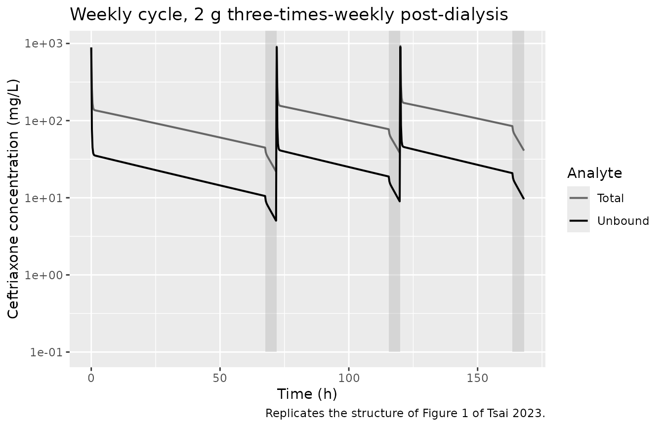
Replicates the structure of Figure 1 of Tsai 2023: typical-value total and unbound ceftriaxone across one weekly cycle of the 2 g three-times-weekly post-dialysis regimen. Shaded bands are dialysis sessions.
Figure 2 – inverse-power clearance versus bilirubin
tibble(TBILI = seq(2, 90, by = 0.5)) |>
  mutate(CL = 0.83 * (14.1 / TBILI)^0.5) |>
  ggplot(aes(TBILI, CL)) +
  geom_line(linewidth = 0.8) +
  geom_vline(xintercept = 14.1, linetype = "dashed", colour = "grey50") +
  annotate("text", x = 14.1, y = 1.9, label = "reference 14.1 umol/L",
           hjust = -0.05, size = 3, colour = "grey30") +
  labs(x = "Serum bilirubin (umol/L)", y = "Interdialytic clearance CL (L/h)",
       title = "CL = CLnHD * (14.1 / bilirubin)^0.5",
       caption = "Replicates Figure 2 of Tsai 2023 (reported r^2 = 0.74).")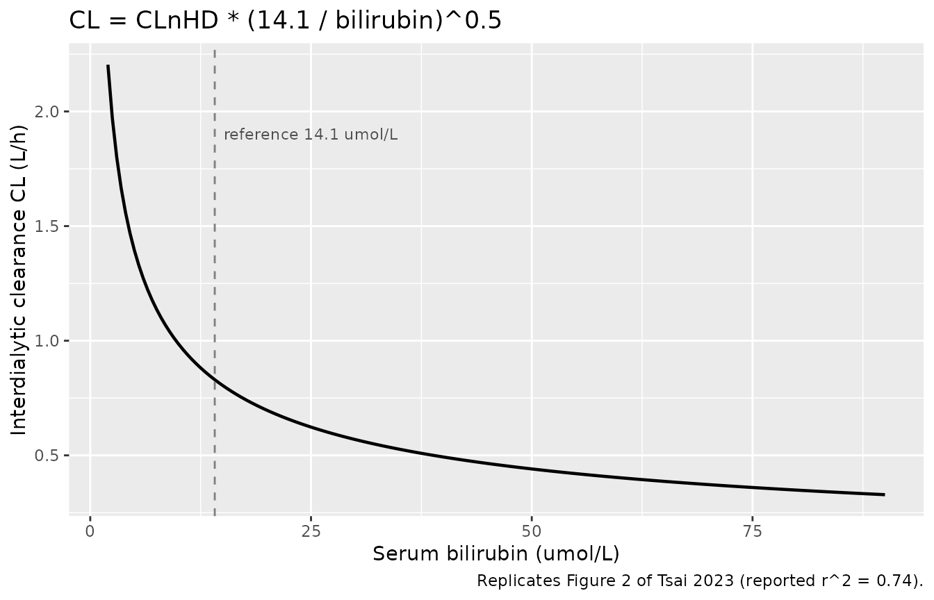
Replicates Figure 2 of Tsai 2023: the inverse-power relationship between interdialytic ceftriaxone clearance and serum bilirubin.
Protein binding
The paper reports a median unbound fraction of 0.29 (IQR 0.20-0.40) – much higher than the 0.04-0.17 typical of healthy individuals. The explicit binding model reproduces this without any fitted unbound-fraction parameter.
fu_df <- sim_72 |>
  filter(time >= 12, Cc > 0) |>
  mutate(fu = Cunbound / Cc)

fu_summary <- tibble(
  Source = c("Simulated", "Tsai 2023 (observed)"),
  Median = c(median(fu_df$fu), 0.29),
  Q1     = c(quantile(fu_df$fu, 0.25), 0.20),
  Q3     = c(quantile(fu_df$fu, 0.75), 0.40)
)

fu_summary |>
  rename("Unbound fraction" = Source, "Q1" = Q1, "Median" = Median, "Q3" = Q3) |>
knitr::kable(digits = 3, caption = "Unbound fraction: simulated vs Tsai 2023 Results.")| Unbound fraction | Median | Q1 | Q3 |
|---|---|---|---|
| Simulated | 0.253 | 0.21 | 0.299 |
| Tsai 2023 (observed) | 0.290 | 0.20 | 0.400 |
ggplot(fu_df, aes(fu)) +
  geom_histogram(bins = 50, fill = "grey60", colour = "white") +
  geom_vline(xintercept = c(0.20, 0.29, 0.40), linetype = c(3, 1, 3)) +
  labs(x = "Unbound fraction", y = "Count",
       title = "Simulated unbound fraction",
       caption = "Solid line = Tsai 2023 median 0.29; dotted = reported IQR 0.20-0.40.")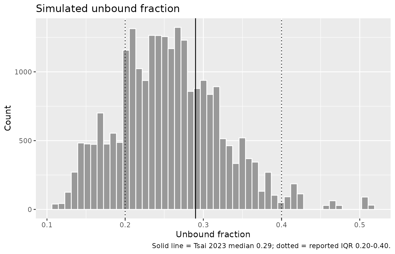
Simulated unbound fraction over the interdialytic interval versus the values reported by Tsai 2023.
Dialysis effect
Two reported quantities probe the dialysis switch: clearance is > 10-fold higher during a session, and unbound concentrations fall by a median 70% (IQR 64-74%) across each session.
# Clearance ratio at the reference bilirubin.
c(CLnHD = 0.83, CLHD = 8.76, ratio = 8.76 / 0.83)
#>    CLnHD     CLHD    ratio
#>  0.83000  8.76000 10.55422

# 4.5 h session beginning 48 h after a 2 g dose.
ev_hd <- make_events(cohort, dose_mg = 2000, dose_times = 0,
                     obs_times = sort(unique(c(seq(0, 72, by = 0.5), 48, 48 + SESSION_H))),
                     sessions = list(c(48, 48 + SESSION_H)), label = "with dialysis")
sim_hd <- rxode2::rxSolve(mod, events = ev_hd, sigma = NA, keep = "treatment") |>
  as.data.frame()

reduction <- sim_hd |>
  filter(time %in% c(48, 48 + SESSION_H)) |>
  group_by(id) |>
  summarise(pct = 100 * (1 - Cunbound[time == 48 + SESSION_H] / Cunbound[time == 48]),
            .groups = "drop")

tibble(
  Quantity = c("Simulated", "Tsai 2023 (observed)"),
  Median   = c(median(reduction$pct), 70),
  Q1       = c(quantile(reduction$pct, 0.25), 64),
  Q3       = c(quantile(reduction$pct, 0.75), 74)
) |>
  rename("Unbound reduction per session (%)" = Quantity) |>
  knitr::kable(digits = 1,
caption = "Unbound concentration reduction across one 4.5 h dialysis session.")| Unbound reduction per session (%) | Median | Q1 | Q3 |
|---|---|---|---|
| Simulated | 55.3 | 37.5 | 70.9 |
| Tsai 2023 (observed) | 70.0 | 64.0 | 74.0 |
The simulated median reduction is smaller than the reported 70%; the cause is worked through in Assumptions and deviations below (it stems from the paper’s own half-lives being one-compartment hand calculations, not from a transcription difference).
PKNCA validation
NCA is run on the 72 h interdialytic interval, separately for total and unbound concentrations, stratified by treatment.
sim_nca <- sim_72 |>
  filter(!is.na(Cc)) |>
  select(id, time, Cc, Cunbound, treatment)

# Guarantee a time-zero record per subject so PKNCA can anchor AUC.
sim_nca <- bind_rows(
  sim_nca,
  sim_nca |> distinct(id, treatment) |> mutate(time = 0, Cc = 0, Cunbound = 0)
) |>
  distinct(id, treatment, time, .keep_all = TRUE) |>
  arrange(id, treatment, time)

dose_df <- ev_72 |>
  filter(evid == 1) |>
  select(id, time, amt, treatment)

intervals <- data.frame(
  start = 0, end = Inf,
  cmax = TRUE, tmax = TRUE, auclast = TRUE, half.life = TRUE
)

nca_total <- PKNCA::pk.nca(PKNCA::PKNCAdata(
  PKNCA::PKNCAconc(sim_nca, Cc ~ time | treatment + id),
  PKNCA::PKNCAdose(dose_df, amt ~ time | treatment + id),
  intervals = intervals
))

nca_unbound <- PKNCA::pk.nca(PKNCA::PKNCAdata(
  PKNCA::PKNCAconc(sim_nca, Cunbound ~ time | treatment + id),
  PKNCA::PKNCAdose(dose_df, amt ~ time | treatment + id),
  intervals = intervals
))
summarise_nca <- function(res, analyte) {
  as.data.frame(res) |>
    filter(!is.na(PPORRES), start == 0, end == Inf) |>
    group_by(PPTESTCD) |>
    summarise(Median = median(PPORRES), Q1 = quantile(PPORRES, 0.25),
              Q3 = quantile(PPORRES, 0.75), .groups = "drop") |>
    mutate(Analyte = analyte, .before = 1)
}

bind_rows(summarise_nca(nca_total, "Total"),
          summarise_nca(nca_unbound, "Unbound")) |>
  rename("NCA parameter" = PPTESTCD) |>
  knitr::kable(digits = 2,
caption = "Simulated NCA over the 72 h interdialytic interval (2 g dose).")| Analyte | NCA parameter | Median | Q1 | Q3 |
|---|---|---|---|---|
| Total | adj.r.squared | 1.00 | 1.00 | 1.00 |
| Total | auclast | 5186.03 | 3818.30 | 7011.94 |
| Total | clast.pred | 30.56 | 16.49 | 47.82 |
| Total | cmax | 932.96 | 597.27 | 1374.84 |
| Total | half.life | 39.55 | 21.50 | 73.11 |
| Total | lambda.z | 0.02 | 0.01 | 0.03 |
| Total | lambda.z.n.points | 150.00 | 139.50 | 154.00 |
| Total | lambda.z.time.first | 1.10 | 0.70 | 2.75 |
| Total | lambda.z.time.last | 72.00 | 72.00 | 72.00 |
| Total | r.squared | 1.00 | 1.00 | 1.00 |
| Total | span.ratio | 1.72 | 0.94 | 2.98 |
| Total | tlast | 72.00 | 72.00 | 72.00 |
| Total | tmax | 0.00 | 0.00 | 0.00 |
| Unbound | adj.r.squared | 1.00 | 1.00 | 1.00 |
| Unbound | auclast | 1389.12 | 1028.51 | 1826.66 |
| Unbound | clast.pred | 8.03 | 4.41 | 11.59 |
| Unbound | cmax | 932.96 | 597.27 | 1374.84 |
| Unbound | half.life | 37.23 | 20.23 | 68.42 |
| Unbound | lambda.z | 0.02 | 0.01 | 0.03 |
| Unbound | lambda.z.n.points | 150.00 | 142.75 | 154.00 |
| Unbound | lambda.z.time.first | 1.10 | 0.70 | 1.83 |
| Unbound | lambda.z.time.last | 72.00 | 72.00 | 72.00 |
| Unbound | r.squared | 1.00 | 1.00 | 1.00 |
| Unbound | span.ratio | 1.87 | 1.02 | 3.13 |
| Unbound | tlast | 72.00 | 72.00 | 72.00 |
| Unbound | tmax | 0.00 | 0.00 | 0.00 |
Comparison against published values
The paper reports no conventional NCA table (no Cmax or AUC), so the
only directly comparable NCA parameter is the interdialytic half-life.
It is compared here with ncaComparisonTable(); the
remaining reported quantities – troughs, unbound fraction and dialysis
reduction – are compared in the table that follows.
published <- tibble::tibble(
  treatment = "2 g post-dialysis",
  half.life = 38.31   # Tsai 2023 Table 2, T(1/2)nHD mean (median 30.40)
)

cmp <- nlmixr2lib::ncaComparisonTable(
  simulated     = nca_unbound,
  reference     = published,
  by            = "treatment",
  params        = "half.life",
  units         = c(half.life = "h"),
  tolerance_pct = 20
)

knitr::kable(cmp, caption = paste(
  "Simulated vs published interdialytic half-life.",
  "* marks a difference of more than 20% from the reference."
))| NCA parameter | treatment | Reference | Simulated | % diff |
|---|---|---|---|---|
| t½ (h) | 2 g post-dialysis | 38.3 | 37.2 | -2.8% |
trough_48 <- sim_72 |> filter(time == 48) |> pull(Cunbound)
trough_72 <- sim_72 |> filter(time == 72) |> pull(Cunbound)

tibble::tribble(
  ~Quantity,                                        ~Simulated,                ~`Tsai 2023 reported`,
  "Unbound trough, 48 h interval (mg/L)",           median(trough_48),         18.2,
  "Unbound trough, 72 h interval (mg/L)",           median(trough_72),         8.8,
  "Unbound fraction",                               median(fu_df$fu),          0.29,
  "Unbound reduction per dialysis session (%)",     median(reduction$pct),     70,
  "Interdialytic clearance at bilirubin 14.1 (L/h)", 0.83,                     0.83,
  "Dialytic / interdialytic clearance ratio",        8.76 / 0.83,              10
) |>
  knitr::kable(digits = 2, caption = paste(
    "Simulated medians versus values reported in Tsai 2023 Results.",
    "Reported IQRs: 48 h trough 9.7-25.9; 72 h trough 7.1-17.7;",
    "unbound fraction 0.20-0.40; session reduction 64-74%."
))| Quantity | Simulated | Tsai 2023 reported |
|---|---|---|
| Unbound trough, 48 h interval (mg/L) | 12.20 | 18.20 |
| Unbound trough, 72 h interval (mg/L) | 8.04 | 8.80 |
| Unbound fraction | 0.25 | 0.29 |
| Unbound reduction per dialysis session (%) | 55.32 | 70.00 |
| Interdialytic clearance at bilirubin 14.1 (L/h) | 0.83 | 0.83 |
| Dialytic / interdialytic clearance ratio | 10.55 | 10.00 |
Both simulated troughs fall inside the reported interquartile ranges, and the simulated unbound fraction sits just below the reported median but inside its IQR. The half-life agrees closely with the reported mean.
Target attainment (Table 3)
The paper’s target is 100% fT > MIC over the final 24 h of a 72 h inter-dialysis interval. Computing the minimum unbound concentration in that window once per subject yields the whole MIC grid from a single simulation per scenario.
pta_scenarios <- tidyr::expand_grid(dose_mg = c(1000, 2000), bili = c(5, 10, 20))

pta_min <- function(dose_mg, bili, idx) {
  subj <- cohort |> mutate(TBILI = bili)
  ev <- make_events(subj, dose_mg = dose_mg, dose_times = 0,
                    obs_times = sort(unique(c(seq(0, 48, by = 2), seq(48, 72, by = 0.5)))),
                    id_offset = as.integer(idx * 1000L),
                    label = paste0(dose_mg / 1000, " g, bili ", bili))
  rxode2::rxSolve(mod, events = ev, sigma = NA, keep = "treatment") |>
    as.data.frame() |>
    filter(time >= 48, time <= 72) |>
    group_by(id, treatment) |>
    summarise(min_fC = min(Cunbound), .groups = "drop")
}

pta_raw <- bind_rows(lapply(seq_len(nrow(pta_scenarios)), function(i) {
  pta_min(pta_scenarios$dose_mg[i], pta_scenarios$bili[i], i) |>
    mutate(dose_mg = pta_scenarios$dose_mg[i], bili = pta_scenarios$bili[i])
}))

mic_grid <- c(0.125, 0.25, 0.5, 1, 2, 4, 8, 16)

pta_tbl <- tidyr::expand_grid(pta_raw, MIC = mic_grid) |>
  group_by(dose_mg, bili, MIC) |>
  summarise(PTA = 100 * mean(min_fC > MIC), .groups = "drop") |>
  mutate(Regimen = paste0(dose_mg / 1000, " g")) |>
  select(Regimen, `Bili (umol/L)` = bili, MIC, PTA) |>
  pivot_wider(names_from = MIC, values_from = PTA)

knitr::kable(pta_tbl, digits = 1, caption = paste(
  "Simulated PTA (%) for 100% fT > MIC over the final 24 h of a 72 h interval.",
  "Compare Tsai 2023 Table 3; see Assumptions for the systematic offset."
))| Regimen | Bili (umol/L) | 0.125 | 0.25 | 0.5 | 1 | 2 | 4 | 8 | 16 |
|---|---|---|---|---|---|---|---|---|---|
| 1 g | 5 | 91.5 | 87.0 | 81.0 | 74.5 | 61.0 | 18.5 | 0.0 | 0 |
| 1 g | 10 | 98.5 | 98.0 | 98.0 | 94.0 | 85.5 | 48.0 | 3.0 | 0 |
| 1 g | 20 | 99.0 | 98.0 | 97.0 | 94.5 | 91.5 | 74.5 | 15.5 | 0 |
| 2 g | 5 | 94.5 | 92.5 | 89.5 | 85.5 | 71.5 | 57.5 | 16.5 | 0 |
| 2 g | 10 | 97.5 | 97.0 | 95.5 | 94.0 | 90.0 | 80.0 | 48.0 | 2 |
| 2 g | 20 | 99.0 | 97.0 | 96.0 | 94.0 | 92.5 | 89.5 | 72.0 | 16 |
Published values for the same cells (Tsai 2023 Table 3, MIC = 1 mg/L): 2 g at bilirubin 5 / 10 / 20 = 97.9 / 100 / 100%; 1 g at bilirubin 5 / 10 / 20 = 86 / 99.5 / 100%. The simulation reproduces the qualitative findings the paper’s recommendations rest on – PTA rises with bilirubin (because clearance falls), 2 g clears the 95% bar where 1 g does not at low bilirubin – but is systematically several points low. The cause is diagnosed below.
Assumptions and deviations
Typical values are Table 2 means. Table 2 reports both a mean and a median for every parameter; the mean column is used here, with the median recorded in each
ini()comment. Pmetrics NPAG estimates a discrete non-parametric distribution, so neither column is a “typical value” in the parametric sense.IIV is a log-normal approximation of a non-parametric distribution. NPAG produces a set of joint support points, not an omega matrix. Table 2 summarises that distribution only by its per-parameter mean, SD and CV%, so the CV% is carried into independent log-normal random effects via
omega^2 = log(CV^2 + 1). The joint structure is unrecoverable from the published summary, and this is the single largest deviation in this extraction. It has a measurable consequence: independent sampling generates parameter combinations that the true support-point distribution would not contain. About 5% of simulated subjects pair a high clearance with a low central volume (median CL 1.90 vs 1.31 L/h and Vc 0.86 vs 2.37 L in that subgroup), giving an implausibly fast elimination rate and a near-zero 72 h concentration. Those subjects fail the PTA target at every MIC, which places a ceiling of roughly 93% on simulated PTA and explains essentially all of the offset from Table 3. The published PTA values should be preferred over the simulated ones; the simulation is included to show the model reproduces the qualitative dose- and bilirubin-dependence, not to restate Table 3.Residual error is the assay polynomial, unscaled. The Table S2
#Errorblock gives an assay-error polynomial of0.3, 0.1, 0, 0for each output (SD = 0.3 + 0.1 * concentration), which is encoded here as a 0.3 mg/L additive plus 10% proportional term on bothCcandCunbound. Pmetrics multiplies that polynomial by an estimated noise-inflation factor gamma; the model file sets only the gamma starting value (G=2) and the final estimated gamma is not reported anywhere in the paper or supplement. The polynomial is therefore carried unscaled (equivalent to gamma = 1), the minimum-assumption reading. If the final gamma were near its starting value, the true residual SD would be about twice what is encoded here.Dialysis session duration is assumed to be 4.5 h. The paper does not state it. 4.5 h is a standard prescription and is used for every figure and table above; no reported quantity was used to select it.
The reported per-session unbound reduction is not reproducible from Table 2’s parameters, and this is a property of the paper rather than of the transcription. Table 2 footnote a marks T(1/2)HD and T(1/2)nHD as “manually calculated”, and they are consistent with the one-compartment formula
0.693 * Vd / CL:0.693 * 36.22 / 8.76 = 2.87 hagainst a reported T(1/2)HD of 3.04 h (median 2.65). A 4.5 h session at a 2.65 h half-life gives a 69% drop, matching the reported 70%. But the model in Table S2 is a three-state system in which elimination acts only on unbound drug in the central compartment, whileKcp / Kpc = 15.37 / 0.78 = 19.7puts about 95% of the drug in the peripheral compartment. During a short session the return flux from the periphery (Kpc = 0.78 1/h) rate-limits the decline, so the model’s true intradialytic half-life is about 5 h and a 4.5 h session removes roughly half the unbound drug rather than 70%. The one-compartment hand calculation therefore understates the model’s intradialytic half-life. Nothing was tuned to close this gap. The same arithmetic explains why Table 2’s Vd of 36.22 L differs fromVc * (1 + Kcp/Kpc) = 46.6 L: the derived rows were computed per support point with a reduced formula, not from the three-state model.The “administered during dialysis” counterfactual is not reproduced. The paper reports a PTA of 0.1% when the 2 g dose is given as a 30 min infusion during the last 30 min of a session. Simulating exactly that – 30 min of dialysis running from the start of the dose, then the session ending – gives a far higher PTA, because fast albumin binding (
k2 = 206 1/h) and fast distribution (k12 = 15.4 1/h) move most of the dose out of the central compartment within minutes, where dialysis cannot reach it. Reproducing 0.1% would require the session to continue for several hours after the dose. Since the supplement does not show howHDxwas set in that simulation, the scenario is omitted rather than guessed at. The paper’s clinical recommendation against dosing during dialysis is not in question – the model does predict substantial intradialytic loss – only the specific 0.1% figure is unreproducible from the published information.Covariates are time-fixed. Serum bilirubin and albumin were treated as time-fixed per subject, as in the source analysis.
TBILIenters as a denominator and must be strictly positive; the virtual cohort floors it at 1 umol/L.Bilirubin reference value. The 14.1 umol/L reference in the clearance covariate is hard-coded in the Table S2 model file and the paper does not state its derivation. It is not the cohort median (10 umol/L). It is carried exactly as printed.
Dose administration. Doses are simulated as bolus inputs into
central. The paper gave each 2 g dose by slow injection within 5 min, which is negligible against a 48-72 h dosing interval. The Pmetrics model file usesRATEIV(1), i.e. an infusion into compartment 1; infusion versus bolus is an event-table choice and requires no model change.