Model and source
#> ℹ parameter labels from comments will be replaced by 'label()'Citation: Qi Y, Chan ML, Mould DR, Larimore K, Fisheleva E, Cherukuri A, Day J, Savarirayan R, Irving M, Bacino CA, Hoover-Fong J, Ozono K, Mohnike K, Wilcox WR, Bober MB, Henshaw J. Development of a weight-band dosing approach for vosoritide in children with achondroplasia using a population pharmacokinetic model. Clin Pharmacokinet. 2024;63(5):707-719. doi:10.1007/s40262-024-01371-6
Description: One-compartment population PK model with first-order elimination and change-point first-order absorption (the absorption rate constant switches from Ka1 to Ka2 at an estimated time after each dose) for subcutaneous vosoritide (BMN 111, a C-type natriuretic peptide analog) in children with achondroplasia aged 0.95-15 years, pooled from five clinical trials (Qi 2024). Body weight is a power covariate on CL/F (exponent 0.356) and on V/F (exponent 1.09), both referenced to 20 kg. Relative bioavailability rises exponentially with time on treatment and is 56% higher for the 0.2 mg/mL dosing solution used only in study 111-202. Study-level random effects nested inside the subject-level IIV on CL/F and V/F reproduce the paper’s secondary study identity number (SIDN) hierarchy, and separate log-scale residual errors are carried for the ELISA and the electrochemiluminescence assays. The model was used to derive the eight-band weight-band dosing regimen of Qi 2024 Table 6.
Vosoritide (BMN 111) is a modified C-type natriuretic peptide analog approved for children with achondroplasia who have open epiphyses. Qi 2024 pooled the plasma PK from five BioMarin trials to build a population PK model and used it to replace the original 15 ug/kg weight-based regimen (17 dose levels between 10 and 83 kg) with an eight-band fixed-dose regimen.
The structural model is one compartment with first-order elimination
and a change-point first-order absorption: the
absorption rate constant is ka1 (2.21 1/h) while time after
dose is below the change-point (0.31 h) and drops to ka2
(0.06 1/h) afterwards. NONMEM implemented the switch with
MTIME.
Simulation requirements for this model
Two things are different from a typical nlmixr2lib model
and both are consequences of the study-level (nested) random
effects:
- The event table must carry a
SIDNcolumn and at least two distinctSIDNvalues.rxode2expands nested random effects into per-level terms; with a single level present the expansion degenerates andrxSolve()fails withThe following parameter(s) are required for solving: THETA[1]. -
omegamust be passed explicitly (omega = mod$omega), both becauserxSolve()otherwise reuses the previous solve’somegaand because the nestedomegais a list of matrices keyed by level.
Independently, every rxSolve() call here passes
useLinCmt = FALSE. rxode2’s automatic
ODE-to-linCmt() conversion would replace the change-point
ODE system with an analytic one-compartment solution evaluated at record
level, which reintroduces the observation-grid dependence the inline
switch exists to avoid.
mod <- mod_ui
mod_typical <- rxode2::zeroRe(mod)
#> Warning: No sigma parameters in the model

#' Solve an event table with the conventions this model requires.
solve_voso <- function(model, events, keep = character()) {
  stopifnot("SIDN" %in% names(events))
  stopifnot(dplyr::n_distinct(events$SIDN) >= 2L)
  rxode2::rxSolve(
    model,
    events = events,
    keep = keep,
    omega = model$omega,
    useLinCmt = FALSE
  ) |>
    as.data.frame()
}

#' Build dosing + observation records for one subject profile.
#' `cmt = "depot"` for the dose and `cmt = "central"` for observations: both
#' are declared ODE states, so `Cc` is returned as a column at the
#' observation rows without triggering compartment renumbering.
make_profile <- function(id, wt, dose_ug, sidn, times = seq(0, 5, by = 1 / 12),
                         soln02 = 0, elisa = 0) {
  dplyr::bind_rows(
    tibble::tibble(time = 0, amt = dose_ug, evid = 1L, cmt = "depot"),
    tibble::tibble(time = times, amt = NA_real_, evid = 0L, cmt = "central")
  ) |>
    dplyr::mutate(
      id = id, WT = wt, SIDN = sidn,
      FORM_VOSO_SOLN02 = soln02, ELISA = elisa
    ) |>
    dplyr::arrange(time, dplyr::desc(evid))
}
Population
The analysis dataset held 4741 plasma vosoritide concentrations from 158 children with achondroplasia enrolled in five trials (Qi 2024 Table 1): study 111-202 (NCT02055157, phase II dose-finding, 2.5 / 7.5 / 15 / 30 ug/kg), its extension 111-205 (NCT02724228), the phase III trial 111-301 (NCT03197766, 15 ug/kg), its extension 111-302 (NCT03424018), and the phase II study 111-206 (NCT03583697) in children 5 years and younger, which contributed interim data from sentinel patients only.
Children were 0.95-15 years old (mean 8.43) and weighed 9-74.5 kg (mean 23.8, median 22.2). 84 were male and 74 female; 114 White, 28 Asian, 6 Black and 10 Other. Doses actually administered were 2.5 ug/kg/day (6 patients), 7.5 ug/kg/day (12), 15 ug/kg/day (151) and 30 ug/kg/day (11). Of the initial 6181 observations, 23.3% were excluded, mostly pre-dose samples that were expected to be non-measurable because vosoritide’s half-life is short relative to once-daily dosing.
The same information is available programmatically through the
model’s population metadata
(readModelDb("Qi_2024_vosoritide")()$population).
Source trace
Every ini() entry in
inst/modeldb/specificDrugs/Qi_2024_vosoritide.R carries an
in-file comment pointing at its source. They are collected here for
review.
| Equation / parameter | Value | Source location |
|---|---|---|
CL/F = exp(theta1 + eta1 + eta6) * (WT/20)^theta14 |
n/a | Qi 2024 Sect. 2.4 covariate equations |
V/F = exp(theta2 + eta2 + eta7) * (WT/20)^theta15 |
n/a | Qi 2024 Sect. 2.4 covariate equations |
Ka1 = exp(theta5 + eta5),
Ka2 = exp(theta6 + eta8)
|
n/a | Qi 2024 Sect. 2.4 |
Change-point = theta7 + eta9; Ka = Ka1 if time after
dose < change-point, else Ka2 |
n/a | Qi 2024 Sect. 2.4 (NONMEM MTIME) |
F = exp(theta16 * Time/10000), Time = h after starting
dose |
n/a | Qi 2024 Sect. 2.4 |
SD1 = theta8, SD2 = theta9
(log-transform-both-sides residual) |
n/a | Qi 2024 Sect. 2.4 |
| Reference body weight | 20 kg | Qi 2024 Sect. 2.4 |
lcl (CL/F) |
47.47 L/h | Qi 2024 Table 5 (%SE 1.8); Table 2 reference row |
lvc (V/F) |
17.99 L | Qi 2024 Table 5 (%SE 3.3); Table 2 reference row |
lka1 (Ka1) |
2.21 1/h | Qi 2024 Table 5 (%SE 14.7) |
lka2 (Ka2) |
0.06 1/h | Qi 2024 Table 5 (%SE 3.8) |
lmtime (change-point) |
0.31 h | Qi 2024 Table 5 (%SE 7.3) |
e_wt_cl |
0.356 | Qi 2024 Table 5 (%SE 25.1); verified against Table 2 |
e_wt_vc |
1.09 | Qi 2024 Table 5 (%SE 8.1); verified against Table 2 |
e_form_voso_soln02_fdepot |
log(1.56) | Qi 2024 Table 5 (%SE 15.3); Table 3 |
e_time_fdepot |
0.21 | Qi 2024 Table 5 (%SE 8.1); verified against Table 4 |
etalcl |
0.336^2 = 0.112896 | Qi 2024 Table 5 IIV CL = 33.6 (CV, %) |
etalvc |
0.242^2 = 0.058564 | Qi 2024 Table 5 IIV V = 24.2 (CV, %) |
etalmtime |
fixed(0.05) |
Qi 2024 Table 5 IIV change-point (fixed) = 22.4 |
etalcl_study |
0.257^2 = 0.066049 | Qi 2024 Table 5 IIV study CL = 25.7 (CV, %) |
etalvc_study |
0.012^2 = 0.000144 | Qi 2024 Table 5 IIV study V = 1.2 (CV, %) |
expSdElisa |
0.665 | Qi 2024 Table 5 Residual error 1 = 66.5, footnote a |
expSdEcl |
0.610 | Qi 2024 Table 5 Residual error 2 = 61, footnote b |
Replicating Qi 2024 Table 2 (weight effect on CL/F and V/F)
Table 2 tabulates the typical CL/F and V/F at 9, 20, 40, 60 and 74.5 kg, both as absolute values and as a percentage of the 20 kg reference. This is an exact deterministic check of the two power covariates.
t2_events <- dplyr::bind_rows(lapply(
  seq_along(c(9, 20, 40, 60, 74.5)),
  function(i) {
    wt <- c(9, 20, 40, 60, 74.5)[i]
    # Two SIDN levels per weight so the nested-eta expansion resolves; with
    # zeroRe() both subjects are identical, and only the first is used.
    dplyr::bind_rows(
      make_profile(2L * i - 1L, wt, 15 * wt, sidn = 1L, times = c(0, 1)),
      make_profile(2L * i, wt, 15 * wt, sidn = 2L, times = c(0, 1))
    ) |>
      dplyr::mutate(WTgroup = wt)
  }
))

t2_sim <- solve_voso(mod_typical, t2_events, keep = "WTgroup")

t2_model <- t2_sim |>
  dplyr::group_by(WTgroup) |>
  dplyr::summarise(cl = dplyr::first(cl), vc = dplyr::first(vc), .groups = "drop") |>
  dplyr::mutate(
    cl_pct = 100 * cl / cl[WTgroup == 20],
    vc_pct = 100 * vc / vc[WTgroup == 20]
  )

t2_published <- tibble::tribble(
  ~WTgroup, ~cl_pub, ~cl_pct_pub, ~vc_pub, ~vc_pct_pub,
  9,        35.72,   75.26,       7.54,    41.88,
  20,       47.47,   100.00,      17.99,   100.00,
  40,       60.75,   127.99,      38.30,   212.87,
  60,       70.18,   147.86,      59.59,   331.18,
  74.5,     75.80,   159.71,      75.45,   419.30
)

t2_published |>
  dplyr::left_join(t2_model, by = "WTgroup") |>
  dplyr::transmute(
    "Body weight (kg)"       = WTgroup,
    "CL/F published (L/h)"   = cl_pub,
    "CL/F model (L/h)"       = round(cl, 2),
    "CL/F published (% ref)" = cl_pct_pub,
    "CL/F model (% ref)"     = round(cl_pct, 2),
    "V/F published (L)"      = vc_pub,
    "V/F model (L)"          = round(vc, 2),
    "V/F published (% ref)"  = vc_pct_pub,
    "V/F model (% ref)"      = round(vc_pct, 2)
  ) |>
knitr::kable(caption = "Replicates Table 2 of Qi 2024.")| Body weight (kg) | CL/F published (L/h) | CL/F model (L/h) | CL/F published (% ref) | CL/F model (% ref) | V/F published (L) | V/F model (L) | V/F published (% ref) | V/F model (% ref) |
|---|---|---|---|---|---|---|---|---|
| 9.0 | 35.72 | 35.72 | 75.26 | 75.26 | 7.54 | 7.53 | 41.88 | 41.88 |
| 20.0 | 47.47 | 47.47 | 100.00 | 100.00 | 17.99 | 17.99 | 100.00 | 100.00 |
| 40.0 | 60.75 | 60.76 | 127.99 | 127.99 | 38.30 | 38.30 | 212.87 | 212.87 |
| 60.0 | 70.18 | 70.19 | 147.86 | 147.86 | 59.59 | 59.58 | 331.18 | 331.18 |
| 74.5 | 75.80 | 75.81 | 159.71 | 159.71 | 75.45 | 75.43 | 419.30 | 419.30 |
Replicating Qi 2024 Tables 3 and 4 (relative bioavailability)
Relative bioavailability rises with time on treatment,
F = exp(0.21 * Time / 10000) with Time in
hours since the first dose (Table 4), and is multiplied by 1.56 when the
0.2 mg/mL dosing solution is used (Table 3). Both are evaluated directly
from the packaged parameters.
f_time <- c(0, 1000, 5000, 10000, 15000, 20000, 25000)
theta <- mod$theta

f_tbl <- tibble::tibble(
  "Time after starting dose (h)"     = f_time,
  "Time after starting dose (years)" = round(f_time / 8766, 2),
  "F, model"                         = round(exp(theta[["e_time_fdepot"]] * f_time / 10000), 2),
  "F, Qi 2024 Table 4"               = c(1.00, 1.02, 1.11, 1.23, 1.37, 1.52, 1.69),
  "F at SOLNC 0.2 mg/mL, model"      = round(
    exp(theta[["e_form_voso_soln02_fdepot"]] + theta[["e_time_fdepot"]] * f_time / 10000), 2
  ),
  "F at SOLNC 0.2 mg/mL, Qi 2024 Table 3" = c(1.56, 1.59, 1.73, 1.92, 2.14, 2.37, 2.64)
)

knitr::kable(f_tbl, caption = "Replicates Tables 3 and 4 of Qi 2024.")| Time after starting dose (h) | Time after starting dose (years) | F, model | F, Qi 2024 Table 4 | F at SOLNC 0.2 mg/mL, model | F at SOLNC 0.2 mg/mL, Qi 2024 Table 3 |
|---|---|---|---|---|---|
| 0 | 0.00 | 1.00 | 1.00 | 1.56 | 1.56 |
| 1000 | 0.11 | 1.02 | 1.02 | 1.59 | 1.59 |
| 5000 | 0.57 | 1.11 | 1.11 | 1.73 | 1.73 |
| 10000 | 1.14 | 1.23 | 1.23 | 1.92 | 1.92 |
| 15000 | 1.71 | 1.37 | 1.37 | 2.14 | 2.14 |
| 20000 | 2.28 | 1.52 | 1.52 | 2.37 | 2.37 |
| 25000 | 2.85 | 1.69 | 1.69 | 2.64 | 2.64 |
Virtual cohort
Individual patient data are not public. Two virtual cohorts are built over the 10-100 kg range of Qi 2024’s simulation:
- the weight-band regimen of Qi 2024 Table 6 (eight fixed doses), and
- the 15 ug/kg per-kg regimen it replaces.
Each of the eight weight bands carries 100 subjects and the 15 ug/kg
arm carries 200, all below the 200-per-arm cap. Body weights are drawn
uniformly inside each band. SIDN cycles over the model’s
three study levels.
set.seed(20240423)

bands <- tibble::tribble(
  ~band,      ~wt_lo, ~wt_hi, ~dose_mg,
  "10-11 kg",  10,     11,     0.24,
  "12-16 kg",  12,     16,     0.28,
  "17-21 kg",  17,     21,     0.32,
  "22-32 kg",  22,     32,     0.40,
  "33-43 kg",  33,     43,     0.50,
  "44-59 kg",  44,     59,     0.60,
  "60-89 kg",  60,     89,     0.70,
  ">= 90 kg",  90,     100,    0.80
)

n_band <- 100L
n_perkg <- 200L

band_events <- dplyr::bind_rows(lapply(seq_len(nrow(bands)), function(i) {
  b <- bands[i, ]
  wts <- stats::runif(n_band, b$wt_lo, b$wt_hi)
  ids <- (i - 1L) * n_band + seq_len(n_band)
  dplyr::bind_rows(lapply(seq_len(n_band), function(j) {
    make_profile(ids[j], wts[j], b$dose_mg * 1000, sidn = (ids[j] %% 3L) + 1L)
  })) |>
    dplyr::mutate(band = b$band, regimen = "Weight band")
}))

#' Which Table 6 weight band does a weight fall into?
band_of <- function(wt) {
  bands$band[max(which(bands$wt_lo <= wt))]
}

perkg_events <- {
  ids <- 10000L + seq_len(n_perkg)
  wts <- stats::runif(n_perkg, 10, 100)
  dplyr::bind_rows(lapply(seq_len(n_perkg), function(j) {
    make_profile(ids[j], wts[j], 15 * wts[j], sidn = (ids[j] %% 3L) + 1L) |>
      dplyr::mutate(band = band_of(wts[j]))
  })) |>
    dplyr::mutate(regimen = "15 ug/kg")
}

events <- dplyr::bind_rows(band_events, perkg_events)
stopifnot(!anyDuplicated(unique(events[, c("id", "time", "evid")])))
stopifnot(dplyr::n_distinct(events$SIDN) >= 2L)
Simulation
sim <- solve_voso(mod, events, keep = c("band", "regimen", "WT"))
stopifnot(dplyr::n_distinct(sim$id) == dplyr::n_distinct(events$id))
The subject-count assertion is deliberate: rxSolve() has
been observed to drop subjects silently on large population solves.
Concentration-time profiles
sim |>
  dplyr::filter(!is.na(Cc), regimen == "Weight band") |>
  dplyr::mutate(band = factor(band, levels = bands$band)) |>
  dplyr::group_by(band, time) |>
  dplyr::summarise(
    Q05 = stats::quantile(Cc, 0.05),
    Q50 = stats::quantile(Cc, 0.50),
    Q95 = stats::quantile(Cc, 0.95),
    .groups = "drop"
  ) |>
  ggplot(aes(time, Q50)) +
  geom_ribbon(aes(ymin = Q05, ymax = Q95), alpha = 0.25) +
  geom_line() +
  facet_wrap(~band) +
  labs(
    x = "Time after dose (h)", y = "Vosoritide concentration (ug/L)",
    title = "Simulated day-1 profiles under the Qi 2024 weight-band regimen",
    caption = "Median with 5th-95th percentile band; 100 subjects per weight band."
  )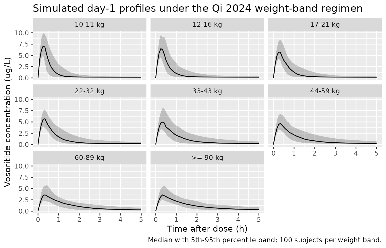
The absorption change-point at 0.31 h is visible as the kink at the peak: below it absorption runs at 2.21 1/h, above it at 0.06 1/h, so the profile turns over sharply and then declines under the slow-absorption (flip-flop) tail.
PKNCA validation
sim_nca <- sim |>
  dplyr::filter(!is.na(Cc)) |>
  dplyr::select(id, time, Cc, band, regimen)

# Guarantee a time = 0 record per subject; vosoritide is given
# subcutaneously, so the pre-dose concentration is 0.
sim_nca <- dplyr::bind_rows(
  sim_nca,
  sim_nca |>
    dplyr::distinct(id, band, regimen) |>
    dplyr::mutate(time = 0, Cc = 0)
) |>
  dplyr::distinct(id, time, .keep_all = TRUE) |>
  dplyr::arrange(regimen, band, id, time)

conc_obj <- PKNCA::PKNCAconc(sim_nca, Cc ~ time | regimen + band + id)

dose_df <- events |>
  dplyr::filter(evid == 1) |>
  dplyr::select(id, time, amt, band, regimen)

dose_obj <- PKNCA::PKNCAdose(dose_df, amt ~ time | regimen + band + id)

intervals <- data.frame(
  start = 0, end = 5,
  cmax = TRUE, tmax = TRUE, auclast = TRUE
)

nca_res <- PKNCA::pk.nca(
  PKNCA::PKNCAdata(conc_obj, dose_obj, intervals = intervals)
)
Exposure consistency across the weight range
Qi 2024 Figures 3 and 4 make the case for the weight-band regimen by showing that its simulated AUC and Cmax sit inside the range observed at 15 ug/kg while being more consistent across body weight. The same contrast is reproduced here.
nca_df <- as.data.frame(nca_res) |>
  dplyr::filter(PPTESTCD %in% c("cmax", "auclast")) |>
  dplyr::mutate(
    band = factor(band, levels = bands$band),
    PPTESTCD = dplyr::recode(
      PPTESTCD,
      cmax = "Cmax (ug/L)", auclast = "AUC0-5h (ug*h/L)"
    )
  )

ggplot(nca_df, aes(band, PPORRES, fill = regimen)) +
  geom_boxplot(outlier.size = 0.4, position = position_dodge(preserve = "single")) +
  facet_wrap(~PPTESTCD, scales = "free_y", ncol = 1) +
  labs(
    x = "Body-weight band", y = NULL,
    title = "Weight-band vs 15 ug/kg exposure",
    caption = "Replicates the comparison in Figures 3 and 4 of Qi 2024."
  ) +
  theme(axis.text.x = element_text(angle = 30, hjust = 1),
        legend.position = "top")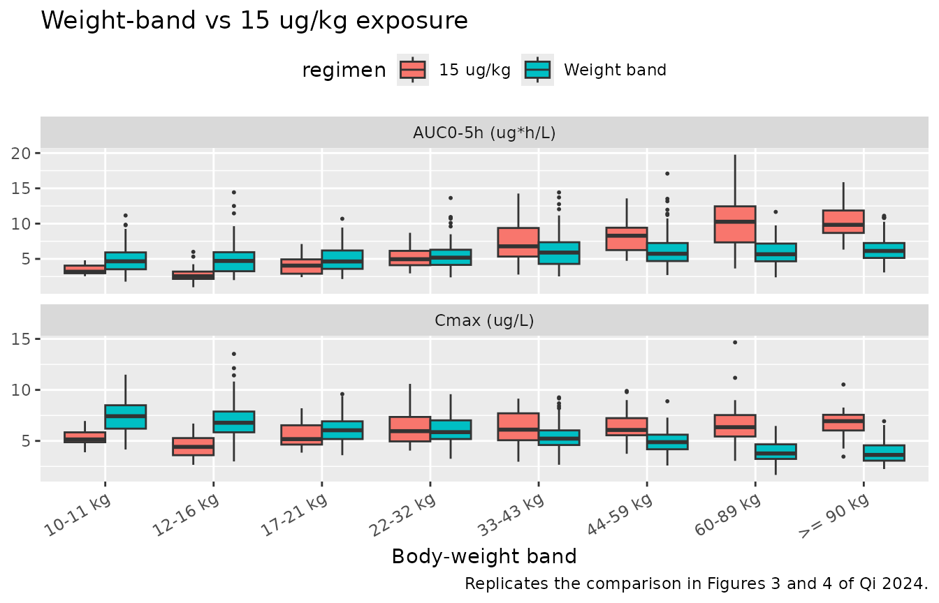
nca_df |>
  dplyr::group_by(regimen, PPTESTCD) |>
  dplyr::summarise(
    median = stats::median(PPORRES),
    p05 = stats::quantile(PPORRES, 0.05),
    p95 = stats::quantile(PPORRES, 0.95),
    .groups = "drop"
  ) |>
  dplyr::mutate(fold_5_95 = round(p95 / p05, 2)) |>
  dplyr::transmute(
    Regimen = regimen,
    "NCA parameter" = PPTESTCD,
    Median = round(median, 3),
    "5th pctile" = round(p05, 3),
    "95th pctile" = round(p95, 3),
    "95th / 5th" = fold_5_95
  ) |>
  knitr::kable(
    caption = paste(
      "Spread of simulated exposure across the whole 10-100 kg range.",
      "A smaller 95th/5th ratio means more consistent exposure."
    )
)| Regimen | NCA parameter | Median | 5th pctile | 95th pctile | 95th / 5th |
|---|---|---|---|---|---|
| 15 ug/kg | AUC0-5h (ug*h/L) | 8.315 | 2.867 | 15.344 | 5.35 |
| 15 ug/kg | Cmax (ug/L) | 5.830 | 3.708 | 8.817 | 2.38 |
| Weight band | AUC0-5h (ug*h/L) | 5.704 | 3.128 | 10.486 | 3.35 |
| Weight band | Cmax (ug/L) | 5.270 | 2.806 | 8.704 | 3.10 |
Comparison against published NCA
Qi 2024’s Introduction reports the non-compartmental parameters observed after a single subcutaneous 15 ug/kg dose across two of the pooled trials: Cmax 4750-7180 pg/mL, AUC from time 0 to the last measurable concentration 175,000-290,000 pgmin/mL, terminal half-life 21.0-27.9 min, and Tmax 13.8-16.8 min. Converted to this model’s units (1 pg/mL = 0.001 ug/L, 1 pgmin/mL = 1.667e-5 ugh/L) those become Cmax 4.75-7.18 ug/L, AUClast 2.92-4.83 ugh/L and Tmax 0.23-0.28 h. The midpoint of each published range is used as the reference value.
The comparator is the typical-value profile of a 20 kg child (the model’s reference weight) given 15 ug/kg = 300 ug.
typ_events <- dplyr::bind_rows(
  make_profile(1L, 20, 300, sidn = 1L, times = seq(0, 5, by = 1 / 60)),
  make_profile(2L, 20, 300, sidn = 2L, times = seq(0, 5, by = 1 / 60))
) |>
  dplyr::mutate(regimen = "15 ug/kg, 20 kg child")

typ_sim <- solve_voso(mod_typical, typ_events, keep = "regimen") |>
  dplyr::filter(id == 1)

typ_nca_conc <- typ_sim |>
  dplyr::filter(!is.na(Cc)) |>
  dplyr::select(id, time, Cc, regimen)

typ_nca_conc <- dplyr::bind_rows(
  typ_nca_conc,
  typ_nca_conc |>
    dplyr::distinct(id, regimen) |>
    dplyr::mutate(time = 0, Cc = 0)
) |>
  dplyr::distinct(id, time, .keep_all = TRUE) |>
  dplyr::arrange(id, time)

typ_dose <- typ_events |>
  dplyr::filter(evid == 1, id == 1) |>
  dplyr::select(id, time, amt, regimen)

typ_nca <- PKNCA::pk.nca(PKNCA::PKNCAdata(
  PKNCA::PKNCAconc(typ_nca_conc, Cc ~ time | regimen + id),
  PKNCA::PKNCAdose(typ_dose, amt ~ time | regimen + id),
  intervals = data.frame(start = 0, end = 5, cmax = TRUE, tmax = TRUE, auclast = TRUE)
))
published <- tibble::tribble(
  ~regimen,                 ~cmax,               ~tmax,               ~auclast,
  "15 ug/kg, 20 kg child",  mean(c(4.75, 7.18)), mean(c(0.23, 0.28)), mean(c(2.92, 4.83))
)

nlmixr2lib::ncaComparisonTable(
  simulated = typ_nca,
  reference = published,
  by = "regimen",
  units = c(cmax = "ug/L", tmax = "h", auclast = "ug*h/L"),
  tolerance_pct = 20
) |>
  knitr::kable(
    caption = paste(
      "Simulated typical-value NCA vs the midpoint of the single-dose",
      "15 ug/kg ranges reported in Qi 2024's Introduction.",
      "* marks a difference greater than 20%."
    ),
    align = c("l", "l", "r", "r", "r")
)| NCA parameter | regimen | Reference | Simulated | % diff |
|---|---|---|---|---|
| Cmax (ug/L) | 15 ug/kg, 20 kg child | 5.96 | 5.35 | -10.4% |
| Tmax (h) | 15 ug/kg, 20 kg child | 0.255 | 0.3 | +17.6% |
| AUClast (ug*h/L) | 15 ug/kg, 20 kg child | 3.88 | 3.86 | -0.4% |
Cmax and AUClast fall inside the published ranges. Tmax is pinned at the absorption change-point (0.31 h), a little later than the observed 0.23-0.28 h window; the paper itself notes that the model underestimates Cmax relative to the observed data (Sect. 3.4 and Discussion limitations), which is the same structural feature seen from the other side.
Terminal half-life is deliberately not compared. With
ka2 (0.06 1/h) far below kel
(CL/F / (V/F) = 2.64 1/h at 20 kg) the model is in
flip-flop, so a terminal slope taken from the model’s tail reflects the
slow absorption phase (t-half about 11.6 h) rather than the 21-28 min
disposition half-life that the sampling window of the source studies
captured.
Assumptions and deviations
-
Scale of the Table 5 “(CV, %)” column. Table 5
reports every variability term under one “(CV, %)” heading without
saying whether the number is
100 * sqrt(omega^2)or an exact log-normal CV. The change-point row settles it: it is the only fixed variance in the table (22.4, %SE 0, bootstrap NE), and100 * sqrt(0.05) = 22.36rounds to 22.4 for a round fixedomega^2of 0.05, whereas the exact log-normal back-transform100 * sqrt(exp(0.05) - 1) = 22.6does not match. Every percentage in Table 5 is therefore read here as100 x SDon the parameter’s own scale, soomega^2 = (CV/100)^2and the residual SDs areCV/100. That reading also agrees with the paper’s own equations, which name the residual quantities standard deviations (SD1 = theta8,SD2 = theta9) rather than CVs. Under the alternativeomega^2 = log(1 + CV^2)convention the IIV variances would be up to 6% smaller and the residual SDs would be 0.605 and 0.562. -
Change-point parameterisation. Qi 2024 prints
Change-point = theta7 + eta9, i.e. an additive random effect. Taken literally together with the fixed 22.4% variability that is an additive SD of 0.224 h on a 0.31 h change-point, a 72% relative spread that would be negative for roughly 8% of subjects. The model file encodes the change-point log-normally (lmtimewithetalmtime ~ fixed(0.05)), which reproduces the reported 22.4% spread (SD 0.0693 h vs 0.0694 h for the additive reading), guarantees positivity, and matches the log-scale parameterisation used for every other structural parameter in the paper. -
SOLNC effect is not in the printed F equation. The
Sect. 2.4 equation gives only
F = exp(theta16 * Time/10000). The 1.56 multiplier for the 0.2 mg/mL solution comes from Table 5 and is confirmed by Table 3, whose 0.2 mg/mL column is exactly 1.56 times the Table 4 time-only column at every tabulated time. -
IIV on Ka1 and Ka2 is not carried. The Sect. 2.4
equations show
eta5on Ka1 andeta8on Ka2, but Sect. 3.2 states the model “accounted for the IIV in CL/F, V/F, and change-point” and Table 5 has no Ka IIV rows, so those two etas were not estimated. Ka1 and Ka2 are typical-value only here. -
Study-level random effects.
SIDNis deliberately an opaque integer grouping column. Qi 2024 states there were only three SIDN values in the database but does not say which trials map to which value, so no mapping from study identifier to SIDN level is asserted. Note that Qi 2024’s own simulations were run “with only one SIDN instead of the three SIDNs present in the model” (Sect. 3.4), which the paper offers as one explanation for the simulated Cmax percentiles being narrower than observed. -
Baseline vs time-varying weight. Qi 2024 tested
both baseline and time-varying weight. The paper does not state which
the final model used, so
WTis supplied as a single per-subject value in this vignette; either can be passed. -
Bioavailability grows without bound.
F = exp(0.21 * Time / 10000)has no plateau, so long simulations produce increasingly large relative bioavailability (1.69 at 2.85 years, Table 4). This is faithful to the published model. Qi 2024 cautions in the Discussion that this relationship was informed by a single study (111-205) and that “additional analysis is needed to fully evaluate the relationship between treatment duration and F”. - Virtual cohort. Body weights are drawn uniformly inside each Table 6 weight band rather than from the trial weight distribution, which is not published at that granularity. The >= 90 kg band is capped at 100 kg, matching the 10-90 kg range Qi 2024 simulated.
-
Assay indicator. All simulations here use
ELISA = 0(the electrochemiluminescence assay used in studies 111-206, 111-301 and 111-302, and the one relevant to the weight-band simulation).