Model and source
- Citation: Wei S, Zhang D, Zhao Z, Mei S. Population pharmacokinetic model of vancomycin in postoperative neurosurgical patients. Front Pharmacol. 2022;13:1005791. doi:10.3389/fphar.2022.1005791
- Description: One-compartment IV-infusion population PK model for vancomycin in Chinese adults after neurosurgery (Wei 2022). Clearance scales with a power function of CKD-EPI estimated glomerular filtration rate (exponent 0.80, reference 115.2 mL/min) and of body weight (exponent 0.30, reference 70 kg) and is multiplied by exp(0.13) under concomitant mannitol; the volume of distribution is fixed at 60.2 L from an earlier Chinese neurosurgical model because the trough-dominated data could not estimate it. Exponential IIV on clearance only and combined additive plus proportional residual error.
- Article (open access): https://doi.org/10.3389/fphar.2022.1005791
Wei 2022 is a retrospective population PK analysis of routine therapeutic drug monitoring (TDM) data for intravenous vancomycin at Beijing Tiantan Hospital, fitted in Phoenix NLME 8.3 (FOCE-ELS). The data were dominated by steady-state troughs, so the volume of distribution could not be estimated and was fixed at 60.2 L, the value of an earlier one-compartment model in Chinese neurosurgical adults (Jing et al., J Clin Pharm Ther 2020;45:88-96). Clearance depends on CKD-EPI estimated glomerular filtration rate, body weight and concomitant mannitol.
Population
The model was built on 895 serum concentrations from 560 Chinese adults, 497 of them postoperative neurosurgical patients (Table 1). Age was 52.41 +/- 15.11 years (18-89), body weight 69.74 +/- 13.05 kg (37.5-130), and 370 patients were male and 190 female. CKD-EPI eGFR was 112.74 +/- 30.91 mL/min (3.52-244.48); 68.2% of patients had augmented renal clearance during monitoring and 2.72% had severe renal insufficiency, most of them on renal replacement therapy. Concomitant medications were meropenem (71.32%), mannitol (60.32%) and diuretics (15.95%). Vancomycin was given as 0.5 or 1 g every 6 to 24 hours; the infusion time was not recorded and a 1 h infusion was assumed throughout.
str(readModelDb("Wei_2022_vancomycin")()$population, max.level = 1)
#> List of 16
#>  $ species         : chr "human"
#>  $ n_subjects      : int 560
#>  $ n_studies       : int 1
#>  $ n_concentrations: int 895
#>  $ age_range       : chr "18-89 years"
#>  $ age_mean        : chr "52.41 years (SD 15.11)"
#>  $ weight_range    : chr "37.5-130 kg"
#>  $ weight_mean     : chr "69.74 kg (SD 13.05)"
#>  $ sex_female_pct  : num 33.9
#>  $ race_ethnicity  : chr "Chinese (single centre, Beijing)."
#>  $ disease_state   : chr "Adults treated with intravenous vancomycin with at least one therapeutic-drug-monitoring concentration; 497 of "| __truncated__
#>  $ dose_range      : chr "0.5 or 1 g per dose every 6, 8, 12 or 24 h by intravenous infusion (default 1 h infusion assumed by the authors"| __truncated__
#>  $ regions         : chr "China (Beijing Tiantan Hospital), October 2018 to March 2022."
#>  $ renal_function  : chr "CKD-EPI eGFR mean 112.74 mL/min (SD 30.91, range 3.52-244.48); Cockcroft-Gault CLcr mean 152.94 mL/min (SD 74.8"| __truncated__
#>  $ co_medication   : chr "Meropenem 71.32%, mannitol 60.32%, diuretics (furosemide or torasemide) 15.95%."
#>  $ notes           : chr "Demographics from Wei 2022 Table 1. Retrospective routine TDM data, mostly steady-state troughs (after more tha"| __truncated__
Source trace
Every value below is recorded as an in-file comment next to the
corresponding ini() entry in
inst/modeldb/specificDrugs/Wei_2022_vancomycin.R.
| Equation / parameter | Value | Source location |
|---|---|---|
lcl |
log(7.98) | Table 3, final model: CL = 7.98 L/h (RSE 1.90%); Eq. (5) |
lvc |
fixed(log(60.2)) | Table 3: V = 60.2 L with no RSE or CI; Eq. (6); Methods 2.2.1 (fixed from Jing 2020) |
e_crcl_cl |
0.80 | Table 3 ‘eGFR on CL’ = 0.80 (RSE 4.30%); exponent in Eq. (5) |
e_wt_cl |
0.30 | Table 3 ‘BW on CL’ = 0.30 (RSE 20.19%); exponent in Eq. (5) |
e_conmed_mannitol_cl |
0.13 | Table 3 ‘Mannitol on CL’ = 0.13 (RSE 17.85%); Eq. (5)
e^A, A = 0.13 with mannitol |
etalcl |
0.044983 = log(1 + 0.2145^2) | Table 3 ‘IIV CL (CV%)’ = 21.45; exponential IIV, Eq. (1) |
propSd |
0.25 | Table 3 sigma1 (multiplicative, CV) = 0.25 (RSE 6.45%) |
addSd |
1.51 mg/L | Table 3 sigma2 (additive) = 1.51 mg/L (RSE 25.83%) |
| Reference eGFR 115.2 mL/min | n/a | Denominator in Eq. (5); Methods 2.2.2: continuous covariates centered at the median |
| Reference weight 70 kg | n/a | Denominator in Eq. (5) |
| eGFR equation | n/a | Eq. (4), CKD-EPI with Scr in mg/dL (see Assumptions) |
| One compartment, first-order elimination | n/a | Methods 2.2.1 |
| Combined residual error | n/a | Eq. (2):
Cobs = Cpred + eps * sqrt(1 + (Cpred * sigma1 / sigma2)^2),
i.e. SD = sqrt(sigma2^2 + (sigma1 * Cpred)^2), which is
nlmixr2’s combined2
|
| 1 h IV infusion | n/a | Methods 2.1 and 2.2.4 |
Deterministic checks against the paper’s own arithmetic
mod <- readModelDb("Wei_2022_vancomycin")
ui <- rxode2::rxode(mod)
#> ℹ parameter labels from comments will be replaced by 'label()'
th <- ui$theta
cl_typ <- exp(th[["lcl"]])

checks <- tibble::tibble(
  Quantity = c(
    "Typical CL per kg at 70 kg (L/h/kg)",
    "CL ratio with vs without mannitol"
  ),
  Computed = c(cl_typ / 70, exp(th[["e_conmed_mannitol_cl"]])),
  Published = c(0.11, 1.14),
  `Source (Wei 2022)` = c(
    "Discussion: 'the typical value of vancomycin CL (0.11 L/h/kg)'",
    "Discussion: 'Co-medicated with mannitol resulted in a 14% increase in vancomycin CL'"
  )
)
stopifnot(
  abs(cl_typ / 70 - 0.11) < 0.005,
  abs(exp(th[["e_conmed_mannitol_cl"]]) - 1.14) < 0.005
)
knitr::kable(checks, digits = 3)| Quantity | Computed | Published | Source (Wei 2022) |
|---|---|---|---|
| Typical CL per kg at 70 kg (L/h/kg) | 0.114 | 0.11 | Discussion: ‘the typical value of vancomycin CL (0.11 L/h/kg)’ |
| CL ratio with vs without mannitol | 1.139 | 1.14 | Discussion: ‘Co-medicated with mannitol resulted in a 14% increase in vancomycin CL’ |
Table 4: the published dose-selection simulations
Table 4 of Wei 2022 lists, for six typical patients (eGFR 90, 45 or 15 mL/min; body weight 85 or 65 kg) with and without mannitol, the q12h doses (1 h infusion) that give a steady-state AUC24 of about 400 and of about 600 h*mg/L, together with the simulated AUC24 and its 5th-95th percentile interval from 1,000 Monte Carlo replicates.
table4 <- tibble::tribble(
  ~egfr, ~wt, ~mannitol, ~target, ~dose, ~auc, ~lo, ~hi,
  90, 85, 1, 400, 1600, 401.47, 293.80, 574.70,
  90, 65, 1, 400, 1450, 400.46, 278.89, 563.07,
  45, 85, 1, 400, 900, 402.28, 283.58, 564.73,
  45, 65, 1, 400, 825, 398.85, 275.21, 560.15,
  15, 85, 1, 400, 375, 399.33, 279.04, 541.50,
  15, 65, 1, 400, 350, 399.18, 186.48, 546.08,
  90, 85, 1, 600, 2350, 600.50, 414.31, 844.34,
  90, 65, 1, 600, 2150, 596.63, 425.29, 864.34,
  45, 85, 1, 600, 1350, 600.04, 412.90, 858.12,
  45, 65, 1, 600, 1250, 607.36, 425.11, 848.61,
  15, 85, 1, 600, 560, 596.34, 416.70, 808.63,
  15, 65, 1, 600, 525, 602.02, 422.52, 809.92,
  90, 85, 0, 400, 1400, 402.19, 275.46, 577.10,
  90, 65, 0, 400, 1300, 405.62, 290.79, 567.37,
  45, 85, 0, 400, 800, 401.47, 286.27, 587.27,
  45, 65, 0, 400, 750, 406.38, 283.88, 582.65,
  15, 85, 0, 400, 330, 394.54, 277.72, 528.21,
  15, 65, 0, 400, 310, 398.11, 281.88, 528.18,
  90, 85, 0, 600, 2050, 593.86, 409.72, 834.99,
  90, 65, 0, 600, 1900, 598.44, 424.16, 877.44,
  45, 85, 0, 600, 1200, 607.06, 429.45, 854.37,
  45, 65, 0, 600, 1100, 600.75, 421.69, 847.62,
  15, 85, 0, 600, 500, 593.28, 421.08, 792.91,
  15, 65, 0, 600, 465, 597.17, 422.82, 792.28
) |>
  mutate(
    treatment = sprintf(
      "eGFR %d, %d kg, mannitol %s, %d mg q12h",
      egfr, wt, ifelse(mannitol == 1, "yes", "no"), dose
    )
  )
stopifnot(nrow(table4) == 24, !anyDuplicated(table4$treatment))
Typical-value AUC24
At steady state the AUC over one 24 h day is the daily dose divided by clearance, so the typical-patient AUC24 follows from the encoded parameters in closed form. For a log-normal clearance the cohort median of AUC24 equals this typical value, so it can be compared directly with the Table 4 point values (which carry the paper’s own Monte Carlo noise of roughly 1%).
typ <- table4 |>
  mutate(
    cl = cl_typ * (egfr / 115.2)^th[["e_crcl_cl"]] * (wt / 70)^th[["e_wt_cl"]] *
      exp(th[["e_conmed_mannitol_cl"]] * mannitol),
    auc_typ = 2 * dose / cl,
    pct_diff = 100 * (auc_typ - auc) / auc
  )
# Deterministic on the model side: all 24 cells reproduce within the
# paper's Monte Carlo precision.
stopifnot(all(abs(typ$pct_diff) < 3))
typ |>
  select(egfr, wt, mannitol, dose, auc, auc_typ, pct_diff) |>
  rename(
    "eGFR (mL/min)" = egfr, "Weight (kg)" = wt, "Mannitol" = mannitol,
    "Dose q12h (mg)" = dose, "Table 4 AUC24" = auc,
    "Typical-value AUC24" = auc_typ, "% diff" = pct_diff
  ) |>
knitr::kable(digits = 1, caption = "Typical-value AUC24 (h*mg/L) against Table 4 of Wei 2022.")| eGFR (mL/min) | Weight (kg) | Mannitol | Dose q12h (mg) | Table 4 AUC24 | Typical-value AUC24 | % diff |
|---|---|---|---|---|---|---|
| 90 | 85 | 1 | 1600 | 401.5 | 404.7 | 0.8 |
| 90 | 65 | 1 | 1450 | 400.5 | 397.5 | -0.7 |
| 45 | 85 | 1 | 900 | 402.3 | 396.4 | -1.5 |
| 45 | 65 | 1 | 825 | 398.9 | 393.8 | -1.3 |
| 15 | 85 | 1 | 375 | 399.3 | 397.7 | -0.4 |
| 15 | 65 | 1 | 350 | 399.2 | 402.3 | 0.8 |
| 90 | 85 | 1 | 2350 | 600.5 | 594.4 | -1.0 |
| 90 | 65 | 1 | 2150 | 596.6 | 589.4 | -1.2 |
| 45 | 85 | 1 | 1350 | 600.0 | 594.6 | -0.9 |
| 45 | 65 | 1 | 1250 | 607.4 | 596.7 | -1.8 |
| 15 | 85 | 1 | 560 | 596.3 | 593.9 | -0.4 |
| 15 | 65 | 1 | 525 | 602.0 | 603.5 | 0.2 |
| 90 | 85 | 0 | 1400 | 402.2 | 403.3 | 0.3 |
| 90 | 65 | 0 | 1300 | 405.6 | 405.9 | 0.1 |
| 45 | 85 | 0 | 800 | 401.5 | 401.2 | -0.1 |
| 45 | 65 | 0 | 750 | 406.4 | 407.7 | 0.3 |
| 15 | 85 | 0 | 330 | 394.5 | 398.6 | 1.0 |
| 15 | 65 | 0 | 310 | 398.1 | 405.8 | 1.9 |
| 90 | 85 | 0 | 2050 | 593.9 | 590.5 | -0.6 |
| 90 | 65 | 0 | 1900 | 598.4 | 593.2 | -0.9 |
| 45 | 85 | 0 | 1200 | 607.1 | 601.9 | -0.9 |
| 45 | 65 | 0 | 1100 | 600.8 | 598.0 | -0.5 |
| 15 | 85 | 0 | 500 | 593.3 | 603.9 | 1.8 |
| 15 | 65 | 0 | 465 | 597.2 | 608.7 | 1.9 |
Scale of the clearance IIV
Table 3 reports the clearance IIV only as ‘CV%’ (21.45). For a
log-normal AUC24 the ratio of the 95th to the 5th percentile is
exp(2 * 1.645 * omega), so each Table 4 interval implies an
SD of log-clearance. The encoded
omega = sqrt(log(1 + 0.2145^2)) is set against the
alternative readings of the reported number.
implied_sd <- log(table4$hi / table4$lo) / (2 * qnorm(0.95))
omega_enc <- sqrt(rxode2::rxode(mod)$omega[1, 1])
#> ℹ parameter labels from comments will be replaced by 'label()'
iiv_tab <- tibble::tibble(
  Reading = c(
    "Median SD implied by the 24 Table 4 intervals",
    "Encoded: CV% -> omega^2 = log(1 + CV^2)",
    "Alternative: 21.45% read as omega^2 x 100"
  ),
  `SD of log CL` = c(median(implied_sd), omega_enc, sqrt(0.2145))
)
stopifnot(abs(median(implied_sd) - omega_enc) < 0.02)
knitr::kable(iiv_tab, digits = 3)| Reading | SD of log CL |
|---|---|
| Median SD implied by the 24 Table 4 intervals | 0.211 |
| Encoded: CV% -> omega^2 = log(1 + CV^2) | 0.212 |
| Alternative: 21.45% read as omega^2 x 100 | 0.463 |
The intervals imply an SD of about 0.21, which agrees with the CV reading and rules out a variance reading (which would give intervals more than twice as wide).
Stochastic replication with PKNCA
Each Table 4 cell is simulated as a separate arm of 200 virtual patients with the clearance IIV, given q12h 1 h infusions for 21 days. At eGFR 15 mL/min the half-life is about 27 h, so the run is long enough for every arm to reach steady state. The steady-state AUC24 is computed with PKNCA over the 480-504 h dosing day and compared with the published median.
n_per_arm <- 200
obs_times <- c(0, seq(480, 504, by = 0.5))
dose_times <- seq(0, 492, by = 12)

arm_events <- function(i) {
  arm <- table4[i, ]
  ids <- (i - 1) * n_per_arm + seq_len(n_per_arm)
  doses <- expand.grid(time = dose_times, id = ids)
  doses$evid <- 1L
  doses$amt <- arm$dose
  doses$rate <- arm$dose / 1
  obs <- expand.grid(time = obs_times, id = ids)
  obs$evid <- 0L
  obs$amt <- 0
  obs$rate <- 0
  bind_rows(doses, obs) |>
    mutate(
      cmt = "central",
      CRCL = arm$egfr,
      WT = arm$wt,
      CONMED_MANNITOL = arm$mannitol,
      treatment = arm$treatment
    )
}
events <- bind_rows(lapply(seq_len(nrow(table4)), arm_events)) |>
  arrange(id, time, desc(evid)) |>
  select(id, time, evid, amt, rate, cmt, CRCL, WT, CONMED_MANNITOL, treatment)

rxode2::rxSetSeed(20221005)
sim <- rxode2::rxSolve(
  rxode2::rxode(mod), select(events, -treatment),
  returnType = "data.frame", addCov = TRUE
) |>
  left_join(distinct(events, id, treatment), by = "id")
#> ℹ parameter labels from comments will be replaced by 'label()'
stopifnot(!anyNA(sim$Cc), all(sim$Cc >= 0))
conc <- sim |>
  filter(!is.na(Cc)) |>
  select(id, time, Cc, treatment)
dose_df <- events |>
  filter(evid == 1) |>
  select(id, time, amt, treatment)

conc_obj <- PKNCA::PKNCAconc(conc, Cc ~ time | treatment + id)
dose_obj <- PKNCA::PKNCAdose(dose_df, amt ~ time | treatment + id)
intervals <- data.frame(start = 480, end = 504, auclast = TRUE, cmax = TRUE, cmin = TRUE)
nca <- PKNCA::pk.nca(PKNCA::PKNCAdata(conc_obj, dose_obj, intervals = intervals))

auc_sub <- as.data.frame(nca$result) |>
  filter(PPTESTCD == "auclast") |>
  select(id, treatment, auc_nca = PPORRES)
The trapezoidal AUC is first checked against the closed-form
2 * dose / CL for the same simulated subjects; both sides
use identical parameter draws, so the difference is pure numerical
error.
cl_sub <- sim |>
  distinct(id, cl) |>
  left_join(distinct(events, id, treatment), by = "id") |>
  left_join(select(table4, treatment, dose), by = "treatment") |>
  mutate(auc_cf = 2 * dose / cl)
nca_cf <- inner_join(auc_sub, cl_sub, by = c("id", "treatment"))
stopifnot(
  nrow(nca_cf) == nrow(table4) * n_per_arm,
  all(abs(100 * (nca_cf$auc_nca - nca_cf$auc_cf) / nca_cf$auc_cf) < 1)
)
reference <- table4 |>
  select(treatment, auclast = auc)
cmp <- ncaComparisonTable(
  nca, reference,
  by = "treatment", params = "auclast",
  units = c(auclast = "h*mg/L"),
  tolerance_pct = 20
)
knitr::kable(cmp, caption = "Median simulated steady-state AUC24 (480-504 h) against Table 4 of Wei 2022.")| NCA parameter | treatment | Reference | Simulated | % diff |
|---|---|---|---|---|
| AUClast (h*mg/L) | eGFR 90, 85 kg, mannitol yes, 1600 mg q12h | 401 | 409 | +1.9% |
| AUClast (h*mg/L) | eGFR 90, 65 kg, mannitol yes, 1450 mg q12h | 400 | 395 | -1.4% |
| AUClast (h*mg/L) | eGFR 45, 85 kg, mannitol yes, 900 mg q12h | 402 | 398 | -1.0% |
| AUClast (h*mg/L) | eGFR 45, 65 kg, mannitol yes, 825 mg q12h | 399 | 391 | -2.0% |
| AUClast (h*mg/L) | eGFR 15, 85 kg, mannitol yes, 375 mg q12h | 399 | 388 | -2.9% |
| AUClast (h*mg/L) | eGFR 15, 65 kg, mannitol yes, 350 mg q12h | 399 | 398 | -0.3% |
| AUClast (h*mg/L) | eGFR 90, 85 kg, mannitol yes, 2350 mg q12h | 600 | 589 | -1.9% |
| AUClast (h*mg/L) | eGFR 90, 65 kg, mannitol yes, 2150 mg q12h | 597 | 576 | -3.5% |
| AUClast (h*mg/L) | eGFR 45, 85 kg, mannitol yes, 1350 mg q12h | 600 | 609 | +1.6% |
| AUClast (h*mg/L) | eGFR 45, 65 kg, mannitol yes, 1250 mg q12h | 607 | 597 | -1.7% |
| AUClast (h*mg/L) | eGFR 15, 85 kg, mannitol yes, 560 mg q12h | 596 | 597 | +0.1% |
| AUClast (h*mg/L) | eGFR 15, 65 kg, mannitol yes, 525 mg q12h | 602 | 608 | +1.0% |
| AUClast (h*mg/L) | eGFR 90, 85 kg, mannitol no, 1400 mg q12h | 402 | 415 | +3.1% |
| AUClast (h*mg/L) | eGFR 90, 65 kg, mannitol no, 1300 mg q12h | 406 | 396 | -2.3% |
| AUClast (h*mg/L) | eGFR 45, 85 kg, mannitol no, 800 mg q12h | 401 | 394 | -1.9% |
| AUClast (h*mg/L) | eGFR 45, 65 kg, mannitol no, 750 mg q12h | 406 | 406 | -0.0% |
| AUClast (h*mg/L) | eGFR 15, 85 kg, mannitol no, 330 mg q12h | 395 | 406 | +2.9% |
| AUClast (h*mg/L) | eGFR 15, 65 kg, mannitol no, 310 mg q12h | 398 | 402 | +1.0% |
| AUClast (h*mg/L) | eGFR 90, 85 kg, mannitol no, 2050 mg q12h | 594 | 593 | -0.1% |
| AUClast (h*mg/L) | eGFR 90, 65 kg, mannitol no, 1900 mg q12h | 598 | 593 | -0.9% |
| AUClast (h*mg/L) | eGFR 45, 85 kg, mannitol no, 1200 mg q12h | 607 | 586 | -3.5% |
| AUClast (h*mg/L) | eGFR 45, 65 kg, mannitol no, 1100 mg q12h | 601 | 582 | -3.1% |
| AUClast (h*mg/L) | eGFR 15, 85 kg, mannitol no, 500 mg q12h | 593 | 628 | +5.8% |
| AUClast (h*mg/L) | eGFR 15, 65 kg, mannitol no, 465 mg q12h | 597 | 601 | +0.6% |
arm_sum <- auc_sub |>
  group_by(treatment) |>
  summarise(
    sim_med = median(auc_nca),
    sim_lo = quantile(auc_nca, 0.05),
    sim_hi = quantile(auc_nca, 0.95),
    .groups = "drop"
  ) |>
  inner_join(table4, by = "treatment") |>
  mutate(pct_med = 100 * (sim_med - auc) / auc)
stopifnot(
  nrow(arm_sum) == 24,
  # Centre: a mis-transcribed clearance or exponent shifts every arm.
  abs(median(arm_sum$pct_med)) < 3,
  # Envelope over arms, robust to which 200-subject draw lands in the tails.
  quantile(abs(arm_sum$pct_med), 0.9) < 8
)
arm_sum |>
  mutate(
    patient = sprintf("eGFR %d, %d kg", egfr, wt),
    mannitol = ifelse(mannitol == 1, "Mannitol", "No mannitol"),
    target = paste("Target", target)
  ) |>
  ggplot(aes(x = patient)) +
  geom_pointrange(aes(y = auc, ymin = lo, ymax = hi, colour = "Wei 2022 Table 4"),
    position = position_nudge(x = -0.15)
  ) +
  geom_pointrange(aes(y = sim_med, ymin = sim_lo, ymax = sim_hi, colour = "nlmixr2lib simulation"),
    position = position_nudge(x = 0.15)
  ) +
  facet_grid(target ~ mannitol, scales = "free_y") +
  labs(
    x = NULL, y = "Steady-state AUC24 (h*mg/L), median and 5th-95th percentile",
    colour = NULL
  ) +
  theme_bw() +
  theme(axis.text.x = element_text(angle = 30, hjust = 1), legend.position = "bottom")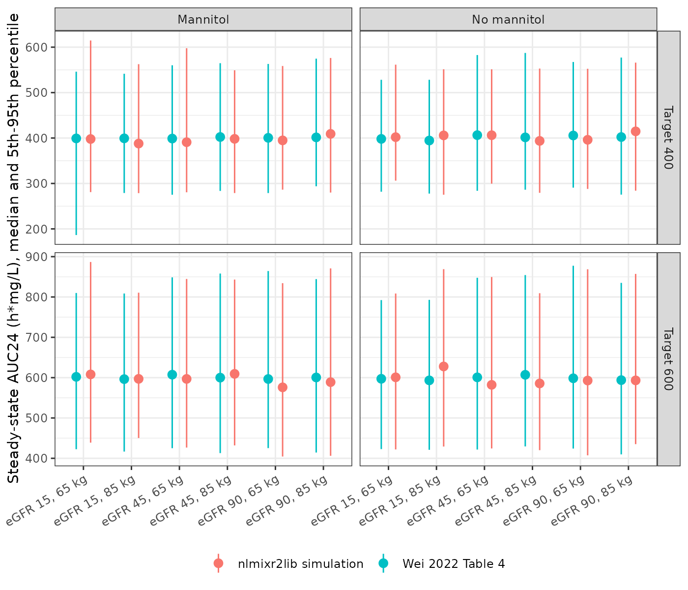
Replicates Table 4 of Wei 2022. The 90% intervals match the published ones in width; the one visible outlier is the published lower bound of 186.48 for the 15 mL/min, 65 kg, mannitol, 350 mg row (see Assumptions and deviations).
Steady-state troughs in a Table 1 cohort
The monitored concentrations were mostly steady-state troughs from a mix of 0.5 g and 1 g regimens given every 6 to 24 hours (mean 14.20 +/- 7.36 mg/L, 20.4% within 15-20 mg/L); the paper does not tabulate how many patients received each regimen. As an illustration, 200 virtual patients with covariates drawn from the Table 1 summaries receive 1 g every 12, 8 or 6 hours (1 h infusions) for 10 days, and the steady-state trough (residual error included) is summarised per regimen. This section is descriptive, not a gate.
set.seed(2022)
n_cohort <- 200
cohort <- tibble::tibble(
  pid = seq_len(n_cohort),
  WT = pmin(pmax(rnorm(n_cohort, 69.74, 13.05), 37.5), 130),
  CRCL = pmin(pmax(rnorm(n_cohort, 112.74, 30.91), 3.52), 244.48),
  CONMED_MANNITOL = rbinom(n_cohort, 1, 0.6032)
)
regimens <- tibble::tibble(regimen = c("1 g q12h", "1 g q8h", "1 g q6h"), tau = c(12, 8, 6))
last_dose <- 216

ev_c <- bind_rows(lapply(seq_len(nrow(regimens)), function(r) {
  tau <- regimens$tau[r]
  arm <- mutate(cohort, id = (r - 1) * n_cohort + pid, regimen = regimens$regimen[r])
  bind_rows(
    tidyr::expand_grid(arm, time = seq(0, last_dose, by = tau)) |>
      mutate(evid = 1L, amt = 1000, rate = 1000),
    tidyr::expand_grid(arm, time = c(0, last_dose + seq(0, tau, by = 0.5))) |>
      mutate(evid = 0L, amt = 0, rate = 0)
  )
})) |>
  mutate(cmt = "central") |>
  arrange(id, time, desc(evid))

rxode2::rxSetSeed(20221006)
sim_c <- rxode2::rxSolve(
  rxode2::rxode(mod),
  select(ev_c, id, time, evid, amt, rate, cmt, CRCL, WT, CONMED_MANNITOL),
  returnType = "data.frame"
) |>
  left_join(distinct(ev_c, id, regimen), by = "id") |>
  left_join(regimens, by = "regimen")
#> ℹ parameter labels from comments will be replaced by 'label()'
trough <- sim_c |> filter(time == last_dose + tau)
stopifnot(nrow(trough) == nrow(regimens) * n_cohort, !anyNA(trough$sim))
trough |>
  group_by(regimen) |>
  summarise(
    `Median trough (mg/L)` = median(sim),
    `5th-95th percentile (mg/L)` = sprintf("%.1f-%.1f", quantile(sim, 0.05), quantile(sim, 0.95)),
    `% in 15-20 mg/L` = 100 * mean(sim >= 15 & sim <= 20),
    .groups = "drop"
  ) |>
  arrange(match(regimen, regimens$regimen)) |>
  rename(Regimen = regimen) |>
knitr::kable(digits = 1)| Regimen | Median trough (mg/L) | 5th-95th percentile (mg/L) | % in 15-20 mg/L |
|---|---|---|---|
| 1 g q12h | 4.4 | 0.3-12.7 | 2 |
| 1 g q8h | 9.3 | 3.3-22.5 | 15 |
| 1 g q6h | 14.5 | 5.6-27.6 | 20 |
sim_c |>
  filter(time >= last_dose) |>
  group_by(regimen, time) |>
  summarise(
    p05 = quantile(sim, 0.05), p50 = median(sim), p95 = quantile(sim, 0.95),
    .groups = "drop"
  ) |>
  mutate(regimen = factor(regimen, levels = regimens$regimen)) |>
  ggplot(aes(time - last_dose, p50)) +
  geom_ribbon(aes(ymin = p05, ymax = p95), alpha = 0.25) +
  geom_line() +
  geom_hline(yintercept = c(15, 20), linetype = "dashed") +
  facet_wrap(~regimen, scales = "free_x") +
  labs(
    x = "Time after the last dose (h)", y = "Vancomycin (mg/L)",
    title = "Steady state in a Table 1 cohort: median and 90% prediction interval"
  ) +
  theme_bw()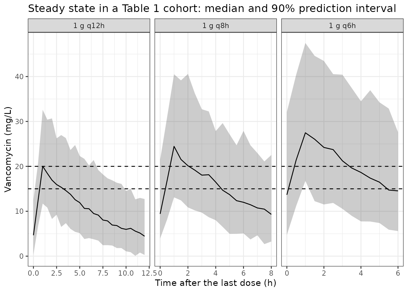
With the typical clearance of 7.98 L/h and the fixed 60.2 L volume, the half-life is about 5.2 h, so a 1 g q12h trough is low (around 4-5 mg/L) even though the corresponding AUC24 is about 240 h*mg/L. The paper’s own Table 4 reaches the same conclusion through AUC24: at eGFR 90 mL/min it needs 1.3-1.6 g q12h for an AUC24 of 400. The observed mean of 14.2 mg/L is matched by the q6h arm here and exceeds the q8h arm. The Supplementary Appendix S2 VPC, which pools all regimens and doses, shows a predicted median near 14 mg/L about 10 h after the dose.
Assumptions and deviations
-
IIV scale. Table 3 reports the clearance IIV only
as ‘21.45 CV%’. It is encoded as
omega^2 = log(1 + 0.2145^2) = 0.044983; the 24 Table 4 AUC24 intervals imply an SD of log-clearance of about 0.21, matching this reading (the variance-times-100 alternative would give SD 0.46). -
eGFR definition. Eq. (4) prints the CKD-EPI
creatinine equation with a 144 multiplier for both sexes, labels the
result mL/min and applies no 1.73 m^2 term. Users should compute
CRCLexactly as printed (Scr in mg/dL) for consistency with the fitted exponent and the 115.2 mL/min reference. The paper reports Table 1 eGFR as a mean (112.74); 115.2 is the median used for centering (Methods 2.2.2). -
Volume fixed from another study. V = 60.2 L comes
from Jing 2020 and was not estimated; it is encoded as
fixed(). No IIV on V was reported, so none is included. - Infusion duration. The paper assumed 1 h infusions because actual infusion times were unavailable; the simulations here do the same.
-
Mannitol flag. The paper does not say whether
mannitol was coded per sample or per patient.
CONMED_MANNITOLcan be supplied either way; the Table 4 simulations hold it constant within a patient. - Probable typo in Table 4. The lower 5% bound for the eGFR 15 mL/min, 65 kg, mannitol, 350 mg q12h row is printed as 186.48, whereas every other 400-target row lies between 275 and 294 and the implied SD for that row alone (0.33) is far from the other 23 (0.19-0.22). It is most likely 286.48. The value is shown as printed and does not enter any assertion other than the median implied SD, which is insensitive to it.
- Trough predictions depend on the borrowed volume. AUC24 depends only on clearance, which the trough-dominated data estimate well (RSE 1.9%). Trough and peak levels also depend on V, which was fixed at the Jing 2020 value rather than estimated, so they carry that study’s uncertainty as well.
- Unretained covariates. Age, height, BMI, serum creatinine, Cockcroft-Gault CLcr, renal replacement therapy, sex, meropenem and diuretics were screened (Table 2) but not retained; no final-model estimates exist for them.