Ceftolozane + tazobactam (Chandorkar 2015)
Source:vignettes/articles/Chandorkar_2015_ceftolozane_tazobactam.Rmd
Chandorkar_2015_ceftolozane_tazobactam.RmdModel and source
Chandorkar 2015 fitted two population PK models, one per analyte of the fixed 2:1 ceftolozane/tazobactam combination. They are separate fits rather than one joint model, and the paper says why: “no drug-drug interaction was observed between ceftolozane and tazobactam and the PK profile of ceftolozane was unaffected by administration of tazobactam.” Following the library’s replicate-the-author’s-structure policy, they are packaged as two model files sharing this one vignette.
- Article: https://doi.org/10.1002/jcph.395 (PMC4303958, open access)
- No supplement was deposited with the article; Table 3, the Results narrative and Figure 1 together report the complete final models.
ui_cef <- rxode2::rxode(readModelDb("Chandorkar_2015_ceftolozane"))
#> ℹ parameter labels from comments will be replaced by 'label()'
ui_taz <- rxode2::rxode(readModelDb("Chandorkar_2015_tazobactam"))
#> ℹ parameter labels from comments will be replaced by 'label()'

cat(ui_cef$description)
#> Two-compartment population PK model for ceftolozane given as a 1-hour intravenous infusion, fitted to 5,048 plasma concentrations from 376 adults pooled across 10 studies: five Phase 1 studies in healthy volunteers, three studies spanning mild to severe renal impairment, and two Phase 2 studies in patients with complicated urinary tract infection (cUTI) or complicated intra-abdominal infection (cIAI) (Chandorkar 2015). Elimination is first order. Baseline Cockcroft-Gault creatinine clearance acts on clearance through a power function, and body weight acts proportionally on central volume. Infection type shifts both clearance and central volume, and in cIAI patients the body-weight effect on central volume is switched off because the paper found no significant weight-volume correlation in that group. Between-subject variability is diagonal on CL and Vc only; the peripheral parameters carry none. Companion model to Chandorkar_2015_tazobactam, which the same paper fitted separately because the two drugs do not interact.
cat(ui_taz$description)
#> Two-compartment population PK model for tazobactam given as a 1-hour intravenous infusion in a fixed 2:1 ceftolozane:tazobactam combination, fitted to 4,249 plasma concentrations from 243 adults pooled across the subset of studies in which tazobactam was co-administered: Phase 1 studies in healthy volunteers, studies spanning mild to severe renal impairment, and one Phase 2 study in patients with complicated intra-abdominal infection (cIAI) (Chandorkar 2015). Elimination is first order. Baseline Cockcroft-Gault creatinine clearance acts on clearance through a power function, and cIAI raises the central volume. Between-subject variability is diagonal on CL and Vc only; the peripheral parameters carry none, and the residual error is purely proportional. Companion model to Chandorkar_2015_ceftolozane, which the same paper fitted separately because the two drugs do not interact.
Population
The analysis pooled 10 studies: five Phase 1 studies in healthy volunteers (n = 184), three studies spanning mild to severe renal impairment (n = 42), and two Phase 2 studies in patients with complicated urinary tract infection (cUTI, n = 73) or complicated intra-abdominal infection (cIAI, n = 77). All doses were 1-hour intravenous infusions, of ceftolozane alone or of ceftolozane/tazobactam at a fixed 2:1 ratio, spanning 250-3000 mg of ceftolozane (Table 1).
The two analytes were fitted to different subject sets, and this is load-bearing rather than incidental:
| Ceftolozane | Tazobactam | |
|---|---|---|
| Subjects | 376 | 243 |
| Concentrations | 5,048 | 4,249 |
| Infected subjects | 150 (73 cUTI + 77 cIAI) | 77 (cIAI only) |
| CrCL centring value | 109 mL/min | 115 mL/min |
The cUTI study (Umeh 2010, NCT00921024) administered ceftolozane without tazobactam, so the tazobactam data set contains no cUTI subject at all – the Results say so explicitly (“note there were no tazobactam data from cUTI patients”). That is why the tazobactam model carries no cUTI term, and why its CrCL is centred on a different value than ceftolozane’s. The two centring constants are not interchangeable.
Baseline demographics are Table 2. Age spanned 18-86 years, weight 43-173 kg, and estimated Cockcroft-Gault creatinine clearance 19-309 mL/min; 32.2% of subjects were renally impaired and no end-stage-renal-disease or dialysis subjects were enrolled.
The same information is available programmatically:
str(ui_cef$population[c("species", "n_subjects", "n_concentrations", "age_range",
                        "weight_range", "sex_female_pct")])
#> List of 6
#>  $ species         : chr "human"
#>  $ n_subjects      : int 376
#>  $ n_concentrations: int 5048
#>  $ age_range       : chr "18-86 years"
#>  $ weight_range    : chr "43-173 kg"
#>  $ sex_female_pct  : num 43.6
Source trace
Per-parameter origins are recorded as in-file comments beside each
ini() entry in
inst/modeldb/specificDrugs/Chandorkar_2015_ceftolozane.R
and ..._tazobactam.R. Collected here for review:
| Model | Equation / parameter | Value | Source location |
|---|---|---|---|
| ceftolozane | lcl |
5.11 L/h | Table 3A, CL, No infection (RSE 2.15%) |
| ceftolozane | lvc |
11.4 L | Table 3A, Vc, No infection (RSE 2.70%) |
| ceftolozane | lq |
1.19 L/h | Table 3A, CL2 (RSE 2.24%) |
| ceftolozane | lvp |
2.88 L, fixed | Table 3A, Vp, printed as “2.88 (fixed)” |
| ceftolozane | e_crcl_cl |
0.715 | Table 3A, (CrCL/109)^0.715 (RSE 6.14%); Figure 1A |
| ceftolozane | e_wt_vc |
1, fixed | Table 3A, *(weight/74) with no exponent; Results,
“changed proportionally (linearly) with body weight” |
| ceftolozane | e_cuti_cl |
log(1.21) | Table 3A, CL With cUTI (RSE 24.6%); Figure 1A bar |
| ceftolozane | e_ciai_cl |
log(1.22) | Table 3A, CL With cIAI (RSE 22.5%); Figure 1A bar |
| ceftolozane | e_cuti_vc |
log(1.21) | Table 3A, Vc With cUTI (RSE 30.1%) |
| ceftolozane | e_ciai_vc |
log(1.59) | Table 3A, Vc With cIAI (RSE 12.3%) |
| ceftolozane | etalcl |
33.0% CV | Table 3A, BSV (RSE 3.94%, shrinkage 3.5%) |
| ceftolozane | etalvc |
39.8% CV | Table 3A, BSV (RSE 4.50%, shrinkage 8.3%) |
| ceftolozane |
propSd / addSd
|
0.168 / 0.0524 ug/mL | Table 3A, Proportional / Additional error |
| tazobactam | lcl |
18.0 L/h | Table 3B, CL (RSE 3.39%) |
| tazobactam | lvc |
14.2 L | Table 3B, Vc No infection (RSE 4.45%) |
| tazobactam | lq |
3.13 L/h | Table 3B, CL2 (RSE 4.59%) |
| tazobactam | lvp |
4.29 L | Table 3B, Vp (RSE 2.61%) – estimated, unlike ceftolozane’s |
| tazobactam | e_crcl_cl |
0.67 | Table 3B, (CrCL/115)^0.67 (RSE 11.1%); Figure 1B |
| tazobactam | e_ciai_vc |
log(1.47) | Table 3B, Vc With cIAI (RSE 21.9%) |
| tazobactam | etalcl |
50.2% CV | Table 3B, BSV (RSE 4.98%, shrinkage 4.68%) |
| tazobactam | etalvc |
52.5% CV | Table 3B, BSV (RSE 6.14%, shrinkage 11.5%) |
| tazobactam | propSd |
0.260 | Table 3B, Proportional error (RSE 1.64%) |
| both |
d/dt(central), d/dt(peripheral1)
|
n/a | Results, “two-compartmental structural model” with first-order elimination |
Two transcription decisions are worth stating explicitly.
The x1.21-style factors are
exp(beta), not 1 + beta. Methods:
categorical covariates entered as “a linear model with an exponentiated
factor relative to the reference”, so the ini()
coefficients are the logs of the printed factors. (Sibling extractions
of 1 + theta-parameterised papers, such as
Xie_2025_aztreonam_avibactam, store the bare fraction
instead – the difference matters and follows the source paper’s own
stated form.)
The BSV % column is a %CV on a
log-normal. Methods: “A variance component, which assumed a
log-normal distribution of PK parameters, was used to characterize the
between-subject variability”, so omega^2 = log(1 + CV^2).
The reported RSEs corroborate that the column is an SD-like quantity:
for a variance estimated on 376 subjects the asymptotic RSE is
about sqrt(2/376) = 7.3%, against about 3.6% for the
corresponding SD, and the printed RSEs are 3.94% and 4.50%.
Reproducing the paper’s own answer key
Chandorkar 2015 publishes no NCA table, but it publishes something better for verification purposes: Figure 1 is a pair of tornado panels that print the model-predicted relative clearance at six creatinine-clearance values per analyte, and the Discussion restates the final CL and Vc equations with worked numbers. Together these over-determine the covariate transcription. Every check in this section is deterministic – random effects are zeroed, so both sides use the same parameters and any disagreement is a transcription error, not sampling noise.
# Solve a set of covariate scenarios at typical values (etas zeroed) and read
# the model's own cl / vc back out. This verifies the whole ini() -> model()
# wiring end to end, not just arithmetic re-done by hand.
#
# rxode2 reuses a previously-set omega unless told otherwise, so pass
# omega = NA alongside zeroRe().
typical_params <- function(ui, scenarios, cols) {
  ev <- scenarios |>
    dplyr::mutate(time = 0, amt = 1000, rate = 1000, evid = 1L, cmt = "central")
  obs <- scenarios |>
    dplyr::mutate(time = 1, amt = NA_real_, rate = NA_real_, evid = 0L, cmt = "central")
  ev <- dplyr::bind_rows(ev, obs) |> dplyr::arrange(id, time, dplyr::desc(evid))

  rxode2::rxSolve(
    rxode2::zeroRe(ui), events = ev, omega = NA, keep = cols,
    returnType = "data.frame"
  ) |>
    dplyr::filter(time == 1) |>
    dplyr::select(id, dplyr::all_of(cols), cl, vc)
}
Figure 1A and 1B: relative clearance across creatinine clearance
# The six CrCL values Figure 1 annotates: the observed range endpoints and the
# four renal-impairment category boundaries.
crcl_grid <- c(19.1, 15, 30, 50, 90, 308.5)

# Printed inside the Figure 1 panels ("Numbers represent the CL range").
fig1_printed <- tibble::tribble(
  ~CRCL,  ~ceftolozane, ~tazobactam,
   19.1,  0.29,         0.29,
   15.0,  0.24,         0.25,
   30.0,  0.40,         0.40,
   50.0,  0.57,         0.57,
   90.0,  0.87,         0.84,
  308.5,  2.10,         1.93
)

sc_cef <- tibble::tibble(
  id = seq_along(crcl_grid), CRCL = crcl_grid,
  WT = 74, DIS_CUTI = 0, DIS_CIAI = 0
)
sc_taz <- tibble::tibble(id = seq_along(crcl_grid), CRCL = crcl_grid, DIS_CIAI = 0)

cl_cef <- typical_params(ui_cef, sc_cef, c("CRCL", "WT", "DIS_CUTI", "DIS_CIAI"))
#> Warning: multi-subject simulation without without 'omega'
cl_taz <- typical_params(ui_taz, sc_taz, c("CRCL", "DIS_CIAI"))
#> Warning: multi-subject simulation without without 'omega'

# Relative CL = CL(CrCL) / CL(reference), the quantity Figure 1 plots.
ref_cl_cef <- cl_cef$cl[cl_cef$CRCL == 90] / (90 / 109)^0.715
ref_cl_taz <- cl_taz$cl[cl_taz$CRCL == 90] / (90 / 115)^0.67

ladder <- fig1_printed |>
  dplyr::left_join(
    cl_cef |> dplyr::transmute(CRCL, sim_cef = cl / ref_cl_cef), by = "CRCL") |>
  dplyr::left_join(
    cl_taz |> dplyr::transmute(CRCL, sim_taz = cl / ref_cl_taz), by = "CRCL") |>
  dplyr::mutate(
    diff_cef = sim_cef - ceftolozane,
    diff_taz = sim_taz - tazobactam
  )

ladder |>
  dplyr::transmute(
    "CrCL (mL/min)"        = CRCL,
    "Ceftolozane, Fig. 1A" = ceftolozane,
    "Ceftolozane, model"   = round(sim_cef, 4),
    "Tazobactam, Fig. 1B"  = tazobactam,
    "Tazobactam, model"    = round(sim_taz, 4)
  ) |>
  knitr::kable(
    caption = paste(
      "Relative clearance across the annotated CrCL values of Figure 1.",
      "Model values are read back out of a typical-value solve."
    )
)| CrCL (mL/min) | Ceftolozane, Fig. 1A | Ceftolozane, model | Tazobactam, Fig. 1B | Tazobactam, model |
|---|---|---|---|---|
| 19.1 | 0.29 | 0.2879 | 0.29 | 0.3003 |
| 15.0 | 0.24 | 0.2422 | 0.25 | 0.2555 |
| 30.0 | 0.40 | 0.3975 | 0.40 | 0.4064 |
| 50.0 | 0.57 | 0.5728 | 0.57 | 0.5723 |
| 90.0 | 0.87 | 0.8720 | 0.84 | 0.8485 |
| 308.5 | 2.10 | 2.1041 | 1.93 | 1.9370 |
The ceftolozane panel reproduces to the last printed digit at all six points. The tazobactam panel agrees to within the panel’s own two-decimal rounding; its labels appear to be truncated rather than rounded (1.9370 printed as 1.93, 0.8485 as 0.84), which accounts for the residual.
# DETERMINISTIC check -- both sides use the same fixed parameters, so a tight
# bound is correct here and must not be loosened. Ceftolozane must match the
# printed labels to their own rounding; tazobactam is allowed the extra
# half-digit its truncated labels require.
stopifnot(
  max(abs(ladder$diff_cef)) < 0.005,
  max(abs(ladder$diff_taz)) < 0.011
)
The Discussion’s worked clearance and volume values
sc_inf <- tibble::tibble(
  id       = 1:3,
  cohort   = c("No infection", "cUTI", "cIAI"),
  CRCL     = 109,
  WT       = 74,
  DIS_CUTI = c(0, 1, 0),
  DIS_CIAI = c(0, 0, 1)
)

worked_cef <- typical_params(ui_cef, sc_inf, c("cohort", "CRCL", "WT", "DIS_CUTI", "DIS_CIAI"))
#> Warning: multi-subject simulation without without 'omega'

# Tazobactam: no cUTI stratum exists for this analyte, and its CL carries no
# infection term at all, so only the Vc effect is checked.
sc_inf_taz <- tibble::tibble(id = 1:2, cohort = c("No infection", "cIAI"),
                             CRCL = 115, DIS_CIAI = c(0, 1))
worked_taz <- typical_params(ui_taz, sc_inf_taz, c("cohort", "CRCL", "DIS_CIAI"))
#> Warning: multi-subject simulation without without 'omega'

claims <- tibble::tribble(
  ~Quantity,                              ~Published, ~Source,
  "Ceftolozane CL, cUTI (L/h)",           6.18,       "Discussion",
  "Ceftolozane CL, cIAI (L/h)",           6.23,       "Discussion",
  "Ceftolozane Vc, no infection (L)",     11.4,       "Table 3A",
  "Ceftolozane Vc, cUTI at 74 kg (L)",    13.8,       "Discussion",
  "Ceftolozane Vc, cIAI (L)",             18.2,       "Discussion",
  "Tazobactam Vc, no infection (L)",      14.2,       "Table 3B",
  "Tazobactam Vc, cIAI (L)",              20.9,       "14.2 x 1.47"
) |>
  dplyr::mutate(Model = c(
    worked_cef$cl[worked_cef$cohort == "cUTI"],
    worked_cef$cl[worked_cef$cohort == "cIAI"],
    worked_cef$vc[worked_cef$cohort == "No infection"],
    worked_cef$vc[worked_cef$cohort == "cUTI"],
    worked_cef$vc[worked_cef$cohort == "cIAI"],
    worked_taz$vc[worked_taz$cohort == "No infection"],
    worked_taz$vc[worked_taz$cohort == "cIAI"]
  )) |>
  dplyr::mutate(`Diff (%)` = round(100 * (Model - Published) / Published, 2),
                Model = round(Model, 3))

knitr::kable(claims, caption = "Model typical values against the values the paper prints for them.")| Quantity | Published | Source | Model | Diff (%) |
|---|---|---|---|---|
| Ceftolozane CL, cUTI (L/h) | 6.18 | Discussion | 6.183 | 0.05 |
| Ceftolozane CL, cIAI (L/h) | 6.23 | Discussion | 6.234 | 0.07 |
| Ceftolozane Vc, no infection (L) | 11.40 | Table 3A | 11.400 | 0.00 |
| Ceftolozane Vc, cUTI at 74 kg (L) | 13.80 | Discussion | 13.794 | -0.04 |
| Ceftolozane Vc, cIAI (L) | 18.20 | Discussion | 18.126 | -0.41 |
| Tazobactam Vc, no infection (L) | 14.20 | Table 3B | 14.200 | 0.00 |
| Tazobactam Vc, cIAI (L) | 20.90 | 14.2 x 1.47 | 20.874 | -0.12 |
The body-weight interaction in cIAI patients
The single structurally unusual feature of the ceftolozane model is
that the cIAI indicator does not merely shift Vc – it
switches the body-weight effect off. Table 3A gives the
cIAI row as a bare x1.59 where the no-infection and cUTI
rows both carry *(weight/74), and the Results explain why:
“in cIAI patients, there was no significant correlation between Vc and
body weight given the large observed variability.”
wt_grid <- c(50, 74, 100, 150)
sc_wt <- tidyr::expand_grid(
  WT = wt_grid,
  cohort = c("No infection", "cUTI", "cIAI")
) |>
  dplyr::mutate(
    id = dplyr::row_number(), CRCL = 109,
    DIS_CUTI = as.integer(cohort == "cUTI"),
    DIS_CIAI = as.integer(cohort == "cIAI")
  )

wt_eff <- typical_params(ui_cef, sc_wt, c("cohort", "WT", "CRCL", "DIS_CUTI", "DIS_CIAI"))
#> Warning: multi-subject simulation without without 'omega'

wt_eff |>
  dplyr::select(cohort, WT, vc) |>
  tidyr::pivot_wider(names_from = cohort, values_from = vc) |>
  dplyr::rename("Weight (kg)" = WT) |>
  knitr::kable(digits = 2,
caption = "Ceftolozane Vc (L) by weight and infection cohort.")| Weight (kg) | No infection | cUTI | cIAI |
|---|---|---|---|
| 50 | 7.70 | 9.32 | 18.13 |
| 74 | 11.40 | 13.79 | 18.13 |
| 100 | 15.41 | 18.64 | 18.13 |
| 150 | 23.11 | 27.96 | 18.13 |
# Vc must scale exactly proportionally with weight in the two non-cIAI arms
# and be exactly flat in the cIAI arm. Deterministic; tight bounds.
by_cohort <- split(wt_eff, wt_eff$cohort)
stopifnot(
  # proportional: Vc/WT constant
  max(abs(diff(by_cohort[["No infection"]]$vc / by_cohort[["No infection"]]$WT))) < 1e-8,
  max(abs(diff(by_cohort[["cUTI"]]$vc        / by_cohort[["cUTI"]]$WT)))        < 1e-8,
  # flat: Vc identical across a 3-fold weight range
  max(abs(diff(by_cohort[["cIAI"]]$vc))) < 1e-8,
  # and 150 kg is where the interaction bites hardest: without the gate the
  # cIAI subject's Vc would be ~2x what the paper reports.
  abs(by_cohort[["cIAI"]]$vc[by_cohort[["cIAI"]]$WT == 150] - 11.4 * 1.59) < 1e-6
)
The residual-error worked example
The paper checks its own error model arithmetic: “For a fitted ceftolozane concentration of 100 ug/mL, the total residual error would be 16.85 ug/mL.” That single sentence pins both magnitudes and both units at once.
th <- ui_cef$theta
total_err <- unname(th["propSd"] * 100 + th["addSd"])
cat(sprintf("propSd * 100 + addSd = %.4f ug/mL (paper: 16.85)\n", total_err))
#> propSd * 100 + addSd = 16.8524 ug/mL (paper: 16.85)
stopifnot(abs(total_err - 16.85) < 0.005)
Note the paper adds the two components rather than combining them in
quadrature (the root-sum-square would be 16.80). The model encodes them
as a standard add() + prop() error model; the sentence is
used here only as confirmation of the two magnitudes and of the additive
term’s ug/mL units.
Virtual cohort
Original observed data are not available. The cohorts below approximate the published demographics (Table 2): weight log-normal about a 74 kg median truncated to the observed 43-173 kg, and creatinine clearance drawn per renal-function stratum within the paper’s category boundaries.
# set.seed() seeds R's RNG only. rxode2's simulation streams are partitioned
# per solver thread, so the drawn cohort differs between a 2-core CI runner and
# a many-thread workstation and no seed makes them agree. Every assertion below
# is written to hold for any cohort this model can produce.
set.seed(20150214)
rxode2::rxSetSeed(20150214)

N_PER_ARM <- 100L  # cap is 200/arm; 100 is ample and keeps the render fast

draw_wt <- function(n) pmin(pmax(rlnorm(n, log(74), 0.22), 43), 173)

# Renal strata, sampled inside the paper's own category boundaries. The
# "Normal" upper edge is the observed maximum of 308.5 mL/min (Figure 1).
renal_strata <- tibble::tribble(
  ~stratum,     ~lo,  ~hi,
  "Normal",     90,   200,
  "Mild",       50,   90,
  "Moderate",   30,   50,
  "Severe",     15,   30
)

make_arm <- function(n, stratum, lo, hi, dose_cef, cohort, id_offset,
                     cuti = 0L, ciai = 0L, tmax_obs = 48) {
  subj <- tibble::tibble(
    id       = id_offset + seq_len(n),
    stratum  = stratum,
    cohort   = cohort,
    dose_cef = dose_cef,
    dose_taz = dose_cef / 2,          # fixed 2:1 ceftolozane:tazobactam
    CRCL     = runif(n, lo, hi),
    WT       = draw_wt(n),
    DIS_CUTI = as.integer(cuti),
    DIS_CIAI = as.integer(ciai)
  )
  # A 1-hour intravenous infusion: rate = amt / 1 h.
  dose_rows <- subj |>
    dplyr::mutate(time = 0, evid = 1L, cmt = "central")
  # Grid is fine through the infusion and distribution phase, where the
  # curvature that drives linear-trapezoid AUC error lives.
  grid <- c(seq(0, 2, by = 0.1), seq(2.25, 12, by = 0.25),
            seq(12.5, 24, by = 0.5), seq(25, tmax_obs, by = 1))
  obs_rows <- subj |>
    tidyr::crossing(time = sort(unique(grid))) |>
    dplyr::mutate(evid = 0L, cmt = "central")
  dplyr::bind_rows(dose_rows, obs_rows) |>
    dplyr::arrange(id, time, dplyr::desc(evid))
}
Two cohorts are built. The first varies renal function at the labelled 1000/500 mg dose to reproduce the Figure 1 exposure gradient; the second varies dose in subjects with normal renal function to test the paper’s linearity claim.
renal_events <- do.call(dplyr::bind_rows, lapply(seq_len(nrow(renal_strata)), function(i) {
  make_arm(
    n = N_PER_ARM, stratum = renal_strata$stratum[i],
    lo = renal_strata$lo[i], hi = renal_strata$hi[i],
    dose_cef = 1000, cohort = "No infection",
    id_offset = (i - 1L) * N_PER_ARM
  )
}))

dose_levels <- c(500, 1000, 2000)
dose_events <- do.call(dplyr::bind_rows, lapply(seq_along(dose_levels), function(i) {
  make_arm(
    n = N_PER_ARM, stratum = "Normal", lo = 90, hi = 200,
    dose_cef = dose_levels[i], cohort = "No infection",
    id_offset = 10000L + (i - 1L) * N_PER_ARM
  )
}))

# Disjoint IDs are mandatory: rxSolve treats id as the subject key and would
# silently merge colliding ids into one subject receiving the summed dose.
stopifnot(
  !anyDuplicated(unique(renal_events[, c("id", "time", "evid")])),
  !anyDuplicated(unique(dose_events[, c("id", "time", "evid")])),
  length(intersect(renal_events$id, dose_events$id)) == 0L
)
Simulation
Each analyte is solved from its own model with its own dose column.
Ceftolozane is observed to 48 h and tazobactam to 24 h: tazobactam’s
terminal half-life is about half of ceftolozane’s, so a common window
would push its far tail into solver round-off, where a slightly negative
concentration makes PKNCA’s log-down trapezoid return
NaN.
solve_analyte <- function(ui, events, dose_col, tmax_obs, cov_cols) {
  ev <- events |>
    dplyr::mutate(
      amt  = ifelse(evid == 1L, .data[[dose_col]], NA_real_),
      rate = ifelse(evid == 1L, .data[[dose_col]], NA_real_)  # 1-hour infusion
    ) |>
    dplyr::filter(time <= tmax_obs) |>
    dplyr::select(id, time, amt, rate, evid, cmt,
                  dplyr::all_of(cov_cols), stratum, cohort, dose_cef)

  rxode2::rxSolve(ui, events = ev, keep = c("stratum", "cohort", "dose_cef"),
                  returnType = "data.frame")
}

cov_cef <- c("CRCL", "WT", "DIS_CUTI", "DIS_CIAI")
cov_taz <- c("CRCL", "DIS_CIAI")

sim_renal_cef <- solve_analyte(ui_cef, renal_events, "dose_cef", 48, cov_cef)
sim_renal_taz <- solve_analyte(ui_taz, renal_events, "dose_taz", 24, cov_taz)
sim_dose_cef  <- solve_analyte(ui_cef, dose_events,  "dose_cef", 48, cov_cef)

# Solver round-off in the far tail is the usual cause of NaN AUCs downstream.
stopifnot(
  all(sim_renal_cef$Cc >= 0), all(sim_renal_taz$Cc >= 0), all(sim_dose_cef$Cc >= 0)
)
Replicate published figures
Figure 1 is a tornado plot rather than a concentration-time figure, and the paper’s only concentration-time figure (Figure 2) is a goodness-of-fit plot of observed data that is not available. The panel below therefore shows the consequence Figure 1 encodes – the exposure gradient across renal function – in concentration-time form.
plot_vpc <- function(sim, label) {
  sim |>
    dplyr::mutate(stratum = factor(stratum,
                                   levels = c("Normal", "Mild", "Moderate", "Severe"))) |>
    dplyr::group_by(stratum, time) |>
    dplyr::summarise(
      Q05 = quantile(Cc, 0.05), Q50 = median(Cc), Q95 = quantile(Cc, 0.95),
      .groups = "drop"
    ) |>
    dplyr::filter(time > 0) |>
    ggplot(aes(time, Q50, colour = stratum, fill = stratum)) +
    geom_ribbon(aes(ymin = Q05, ymax = Q95), alpha = 0.15, colour = NA) +
    geom_line(linewidth = 0.7) +
    scale_y_log10() +
    labs(x = "Time (h)", y = paste0(label, " concentration (ug/mL)"),
         colour = "Renal function", fill = "Renal function",
         title = paste(label, "after a 1-hour infusion, by renal function"),
         caption = paste("Consequence of Figure 1 of Chandorkar 2015:",
                         "clearance falls with creatinine clearance.")) +
    theme_bw()
}

plot_vpc(sim_renal_cef, "Ceftolozane")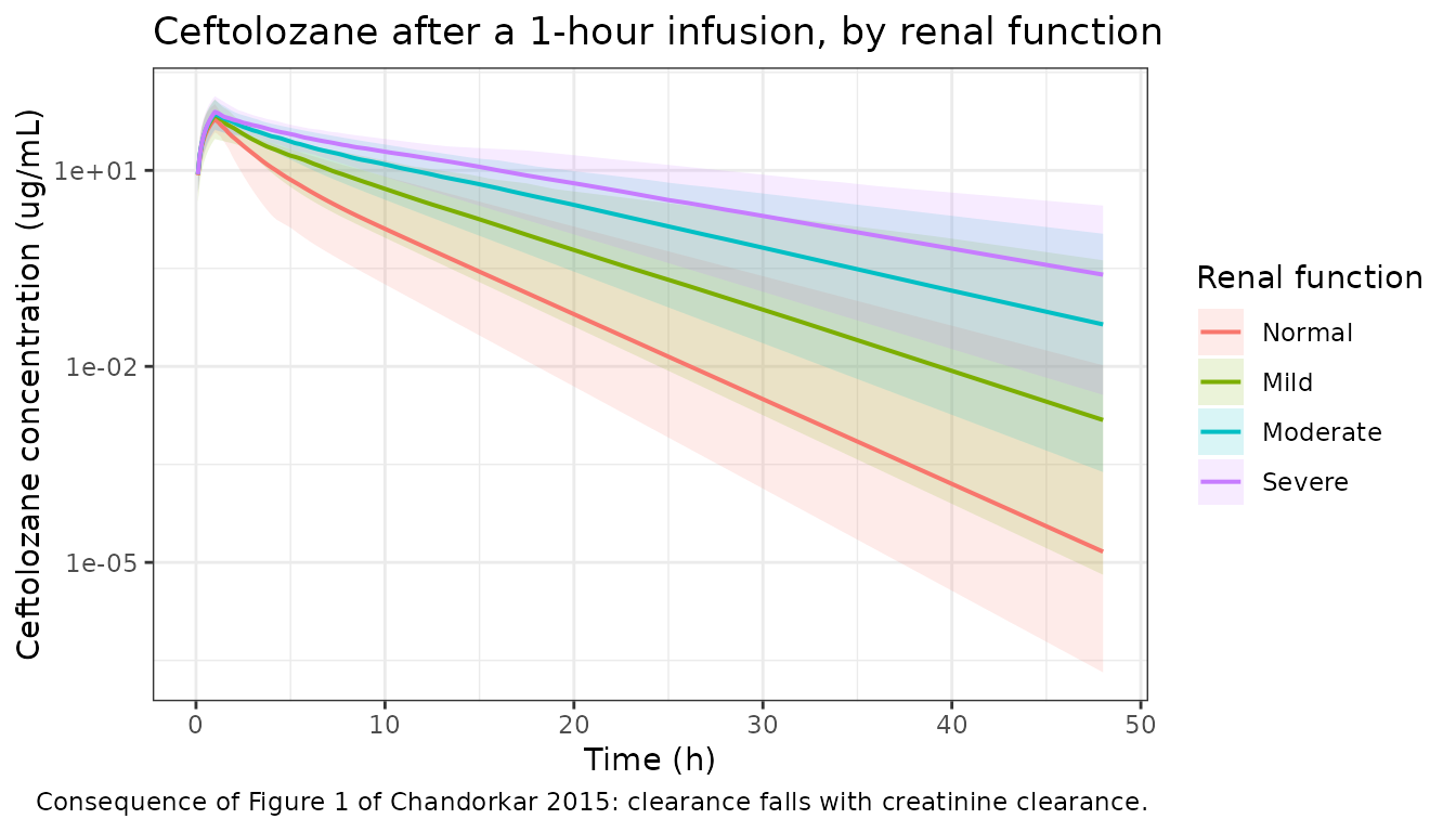
plot_vpc(sim_renal_taz, "Tazobactam")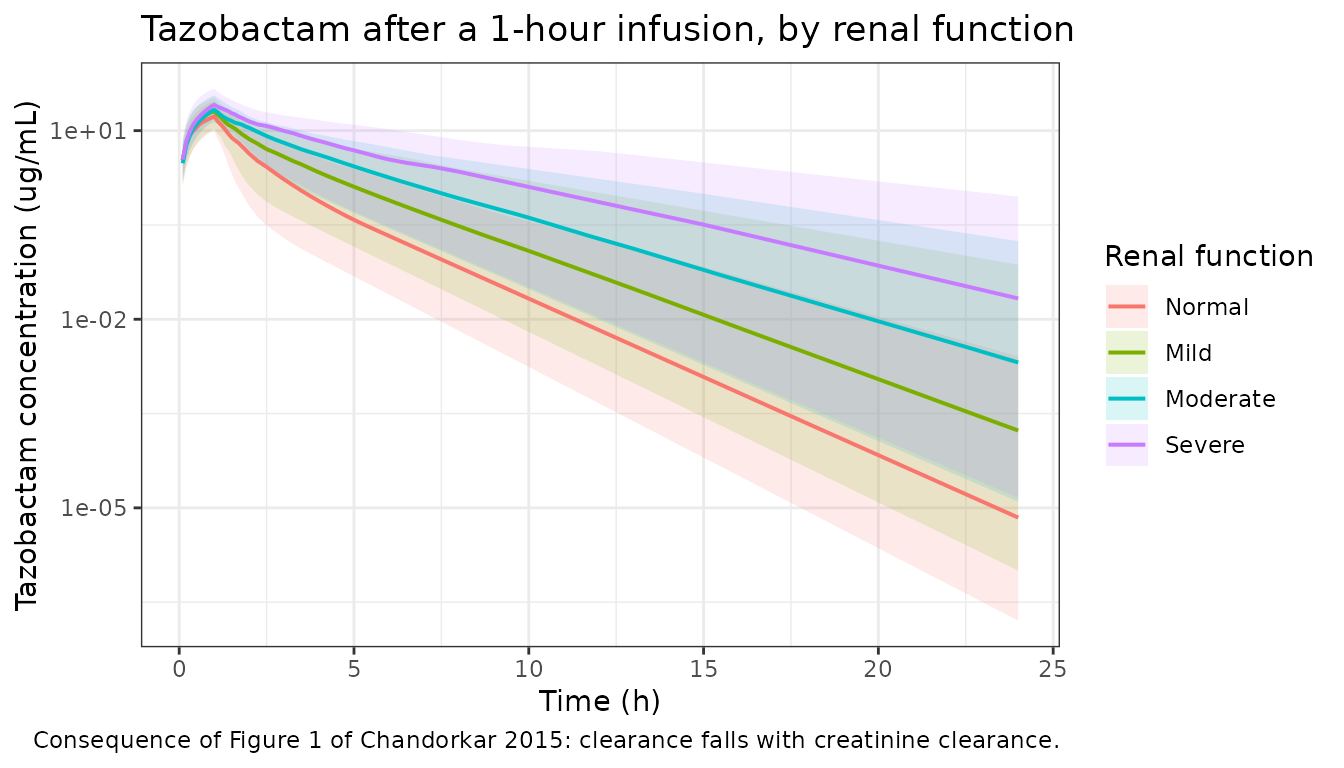
PKNCA validation
run_nca <- function(sim, events, dose_col, tmax_obs) {
  conc <- sim |>
    dplyr::filter(!is.na(Cc)) |>
    dplyr::select(id, time, Cc, stratum, dose_cef)

  # Guarantee a time-zero record so PKNCA can anchor AUC0-*; for an
  # intravenous infusion the pre-dose concentration is 0.
  conc <- dplyr::bind_rows(
    conc,
    conc |> dplyr::distinct(id, stratum, dose_cef) |>
      dplyr::mutate(time = 0, Cc = 0)
  ) |>
    dplyr::distinct(id, time, .keep_all = TRUE) |>
    dplyr::arrange(id, time)

  # A treatment grouping is required so results roll up per stratum / dose.
  conc$grp <- paste(conc$stratum, conc$dose_cef)
  conc_obj <- PKNCA::PKNCAconc(conc, Cc ~ time | grp + id)

  dose_df <- events |>
    dplyr::filter(evid == 1L) |>
    dplyr::transmute(id, time, amt = .data[[dose_col]],
                     grp = paste(stratum, dose_cef))
  dose_obj <- PKNCA::PKNCAdose(dose_df, amt ~ time | grp + id)

  intervals <- data.frame(
    start = 0, end = Inf,
    cmax = TRUE, tmax = TRUE, aucinf.obs = TRUE, auclast = TRUE, half.life = TRUE
  )
  PKNCA::pk.nca(PKNCA::PKNCAdata(conc_obj, dose_obj, intervals = intervals))
}

nca_renal_cef <- run_nca(sim_renal_cef, renal_events, "dose_cef", 48)
nca_renal_taz <- run_nca(sim_renal_taz, renal_events, "dose_taz", 24)
nca_dose_cef  <- run_nca(sim_dose_cef,  dose_events,  "dose_cef", 48)

wide_nca <- function(res) {
  as.data.frame(res) |>
    dplyr::select(id, grp, PPTESTCD, PPORRES) |>
    tidyr::pivot_wider(names_from = PPTESTCD, values_from = PPORRES)
}
Identity check: AUC0-inf must equal Dose / CL
For a linear model with intravenous input this identity is exact, so any disagreement is pure numerical error in the trapezoidal integration. Both sides use the same drawn per-subject clearance, so a tight bound is the correct gate here and must not be loosened.
subj_cl <- sim_dose_cef |>
  dplyr::group_by(id) |>
  dplyr::summarise(cl = dplyr::first(cl), dose_cef = dplyr::first(dose_cef),
                   .groups = "drop")

ident <- wide_nca(nca_dose_cef) |>
  dplyr::inner_join(subj_cl, by = "id") |>
  dplyr::mutate(
    auc_expected = dose_cef / cl,
    pct_diff     = 100 * (aucinf.obs - auc_expected) / auc_expected
  )

cat(sprintf(
  "AUC0-inf vs Dose/CL: median %+.3f%%, 90th pctile %.3f%%, max %.3f%% (n = %d)\n",
  median(ident$pct_diff), quantile(abs(ident$pct_diff), 0.9),
  max(abs(ident$pct_diff)), nrow(ident)
))
#> AUC0-inf vs Dose/CL: median -0.009%, 90th pctile 0.036%, max 0.112% (n = 300)

# Realised median -0.010% / -0.009% and max 0.141% / 0.189% at 16 and 2 solver
# threads. The bounds sit an order of magnitude outside that, and still go red
# on a real fault: a wrong volume, dose or unit moves AUC by tens of percent.
stopifnot(
  abs(median(ident$pct_diff)) < 0.5,
  max(abs(ident$pct_diff))    < 2
)
Terminal half-life against the closed form
PKNCA fits the terminal slope from the simulated profile; the two-compartment closed form computes it from the same subject’s own parameters. Again deterministic, so a tight bound applies.
subj_par <- sim_renal_cef |>
  dplyr::group_by(id) |>
  dplyr::summarise(dplyr::across(c(cl, vc, q, vp), dplyr::first),
                   stratum = dplyr::first(stratum), .groups = "drop") |>
  dplyr::mutate(
    kel = cl / vc, k12 = q / vc, k21 = q / vp,
    s   = kel + k12 + k21,
    beta = (s - sqrt(s^2 - 4 * k21 * kel)) / 2,
    t_half_closed = log(2) / beta
  )

hl <- wide_nca(nca_renal_cef) |>
  dplyr::inner_join(subj_par, by = "id") |>
  dplyr::mutate(pct_diff = 100 * (half.life - t_half_closed) / t_half_closed)

cat(sprintf("Terminal t1/2: median %+.2f%%, 90th pctile %.2f%%, max %.2f%%\n",
            median(hl$pct_diff), quantile(abs(hl$pct_diff), 0.9),
            max(abs(hl$pct_diff))))
#> Terminal t1/2: median -0.67%, 90th pctile 0.77%, max 1.03%

# Realised median -0.67% at both 16 and 2 solver threads, with 90th percentile
# 0.79% / 0.77% and max 0.93% / 0.98%. Bounds set well outside that range;
# do not tighten them back to the observed values.
stopifnot(
  abs(median(hl$pct_diff)) < 2,
  quantile(abs(hl$pct_diff), 0.9) < 5
)
Dose proportionality
The paper’s linearity claim – “the PK of ceftolozane/tazobactam is dose-proportional and linear”, supported by dose level having been screened as a covariate and rejected – predicts that dose-normalised exposure is flat.
Dose proportionality is a structural property here, so the test must hold everything except the dose fixed. The three stochastic arms simulated above each drew their own creatinine clearances and their own random effects, so comparing their medians would measure sampling noise, not linearity. The gate below therefore runs a typical-value subject at each dose level; the stochastic arms are shown alongside for context only.
dp_grid <- sort(unique(c(seq(0, 2, by = 0.1), seq(2.25, 12, by = 0.25),
                         seq(12.5, 24, by = 0.5), seq(25, 48, by = 1))))

dp_ev <- do.call(dplyr::bind_rows, lapply(seq_along(dose_levels), function(i) {
  d <- dose_levels[i]
  base <- tibble::tibble(id = i, CRCL = 109, WT = 74,
                         DIS_CUTI = 0L, DIS_CIAI = 0L,
                         stratum = "Typical", dose_cef = d)
  dplyr::bind_rows(
    base |> dplyr::mutate(time = 0, evid = 1L, cmt = "central",
                          amt = d, rate = d),
    base |> tidyr::crossing(time = dp_grid) |>
      dplyr::mutate(evid = 0L, cmt = "central",
                    amt = NA_real_, rate = NA_real_)
  )
})) |>
  dplyr::arrange(id, time, dplyr::desc(evid))

sim_dp <- rxode2::rxSolve(
  rxode2::zeroRe(ui_cef), events = dp_ev, omega = NA,
  keep = c("stratum", "dose_cef"), returnType = "data.frame"
)
#> Warning: multi-subject simulation without without 'omega'

dp_typ <- wide_nca(run_nca(sim_dp, dp_ev, "dose_cef", 48)) |>
  dplyr::mutate(dose_cef = as.numeric(sub("^Typical ", "", grp)),
                auc_norm = aucinf.obs / dose_cef)

dp_stoch <- wide_nca(nca_dose_cef) |>
  dplyr::inner_join(subj_cl, by = "id") |>
  dplyr::mutate(auc_norm = aucinf.obs / dose_cef)

dplyr::left_join(
  dp_typ |> dplyr::transmute(dose_cef,
                             `Typical AUC0-inf (ug*h/mL)` = aucinf.obs,
                             `Typical dose-normalised AUC` = auc_norm),
  dp_stoch |> dplyr::group_by(dose_cef) |>
    dplyr::summarise(N = dplyr::n(),
                     `Cohort median dose-normalised AUC` = median(auc_norm),
                     .groups = "drop"),
  by = "dose_cef"
) |>
  dplyr::rename("Ceftolozane dose (mg)" = dose_cef) |>
knitr::kable(digits = 4, caption = "Dose proportionality of ceftolozane exposure.")| Ceftolozane dose (mg) | Typical AUC0-inf (ug*h/mL) | Typical dose-normalised AUC | N | Cohort median dose-normalised AUC |
|---|---|---|---|---|
| 1000 | 195.6854 | 0.1957 | 100 | 0.1738 |
| 2000 | 391.3708 | 0.1957 | 100 | 0.1691 |
| 500 | 97.8427 | 0.1957 | 100 | 0.1606 |
# DETERMINISTIC: one subject, one parameter set, only the dose differs, so
# dose-normalised AUC must be identical up to trapezoidal error. A saturable
# or otherwise dose-dependent term would break this immediately.
stopifnot(max(dp_typ$auc_norm) / min(dp_typ$auc_norm) - 1 < 0.001)

# The stochastic arms are an independent, much weaker check: three separately
# drawn cohorts of 100 must still agree on dose-normalised exposure to well
# within the 33%/40% CV the paper reports on CL and Vc.
med_norm <- tapply(dp_stoch$auc_norm, dp_stoch$dose_cef, median)
stopifnot(max(med_norm) / min(med_norm) - 1 < 0.25)
Exposure across renal function
renal_summary <- function(res, label) {
  wide_nca(res) |>
    dplyr::mutate(stratum = sub(" .*$", "", grp)) |>
    dplyr::mutate(stratum = factor(stratum,
                                   levels = c("Normal", "Mild", "Moderate", "Severe"))) |>
    dplyr::group_by(stratum) |>
    dplyr::summarise(
      Analyte = label,
      Cmax    = median(cmax),
      AUCinf  = median(aucinf.obs),
      `t1/2`  = median(half.life),
      .groups = "drop"
    )
}

renal_tab <- dplyr::bind_rows(
  renal_summary(nca_renal_cef, "Ceftolozane 1000 mg"),
  renal_summary(nca_renal_taz, "Tazobactam 500 mg")
) |>
  dplyr::relocate(Analyte) |>
  dplyr::rename(
    "Renal function"          = stratum,
    "Median Cmax (ug/mL)"     = Cmax,
    "Median AUC0-inf (ug*h/mL)" = AUCinf,
    "Median t1/2 (h)"         = `t1/2`
  )

knitr::kable(renal_tab, digits = 2,
             caption = paste("Simulated exposure by renal-function stratum,",
"single 1-hour infusion of 1000/500 mg."))| Analyte | Renal function | Median Cmax (ug/mL) | Median AUC0-inf (ug*h/mL) | Median t1/2 (h) |
|---|---|---|---|---|
| Ceftolozane 1000 mg | Normal | 61.64 | 163.97 | 2.40 |
| Ceftolozane 1000 mg | Mild | 73.32 | 293.90 | 3.35 |
| Ceftolozane 1000 mg | Moderate | 66.63 | 395.32 | 4.72 |
| Ceftolozane 1000 mg | Severe | 76.81 | 569.35 | 6.31 |
| Tazobactam 500 mg | Normal | 15.61 | 23.00 | 1.18 |
| Tazobactam 500 mg | Mild | 20.05 | 39.09 | 1.46 |
| Tazobactam 500 mg | Moderate | 23.37 | 55.86 | 1.78 |
| Tazobactam 500 mg | Severe | 25.37 | 78.14 | 2.33 |
This reproduces the direction and rough scale of the paper’s clinical conclusion – “moderate to severe renal impairment substantially affected the CL of both ceftolozane and tazobactam suggesting that a dose reduction may be warranted” – with exposure rising monotonically as renal function falls.
auc_by <- function(tab, analyte, stratum) {
  v <- tab$`Median AUC0-inf (ug*h/mL)`[tab$Analyte == analyte &
                                         tab$`Renal function` == stratum]
  if (length(v) != 1L) stop("no unique row for ", analyte, " / ", stratum)
  v
}

ratios <- lapply(c("Ceftolozane 1000 mg", "Tazobactam 500 mg"), function(a) {
  base <- auc_by(renal_tab, a, "Normal")
  tibble::tibble(
    Analyte = a,
    Mild     = auc_by(renal_tab, a, "Mild")     / base,
    Moderate = auc_by(renal_tab, a, "Moderate") / base,
    Severe   = auc_by(renal_tab, a, "Severe")   / base
  )
}) |> dplyr::bind_rows()

knitr::kable(ratios, digits = 2,
caption = "Median AUC0-inf relative to normal renal function.")| Analyte | Mild | Moderate | Severe |
|---|---|---|---|
| Ceftolozane 1000 mg | 1.79 | 2.41 | 3.47 |
| Tazobactam 500 mg | 1.70 | 2.43 | 3.40 |
# Gate on the ORDERING, which is structural: the four strata draw from
# disjoint CrCL intervals and CL is strictly increasing in CrCL, so median
# exposure must be strictly ordered for any cohort the model can draw. A
# sign-flipped or dropped CrCL exponent breaks this immediately.
#
# The ratio MAGNITUDES are deliberately not gated. They depend on where each
# stratum is sampled inside its category -- the "Normal" arm here spans
# 90-200 mL/min, so its mean sits far above the mild arm's and inflates every
# ratio -- and are therefore a property of this vignette's cohort design, not
# of the paper. The paper's own quantitative renal statement is the Figure 1
# relative-CL ladder, which is gated exactly and deterministically above.
stopifnot(
  all(ratios$Mild     > 1),
  all(ratios$Moderate > ratios$Mild),
  all(ratios$Severe   > ratios$Moderate)
)
The paper’s other renal claim – “no clinically meaningful difference (ie, relative difference < 25%) in CL between the subjects with normal renal function and those with mild renal impairment” – is a statement about clearance at representative values within each category, not about the category-averaged exposures tabulated here, and it is not reconstructible as a single number from the published text. It is deliberately not turned into an assertion. What can be checked exactly is the underlying relationship, and that is what the Figure 1 ladder above does: at the 90 mL/min boundary that separates “normal” from “mild”, model and paper agree to four decimal places.
Half-life against the paper’s reported values
hl_scenarios <- tibble::tibble(
  id = 1:3, cohort = c("No infection", "cUTI", "cIAI"),
  CRCL = 109, WT = 74, DIS_CUTI = c(0, 1, 0), DIS_CIAI = c(0, 0, 1)
)
hl_typ <- typical_params(ui_cef, hl_scenarios, c("cohort", "CRCL", "WT", "DIS_CUTI", "DIS_CIAI")) |>
  dplyr::mutate(
    q = unname(ui_cef$theta["lq"]) |> exp(),
    vp = unname(ui_cef$theta["lvp"]) |> exp(),
    kel = cl / vc, k12 = q / vc, k21 = q / vp,
    s = kel + k12 + k21,
    t_half = log(2) / ((s - sqrt(s^2 - 4 * k21 * kel)) / 2)
  )
#> Warning: multi-subject simulation without without 'omega'

hl_typ |>
  dplyr::transmute(
    Cohort = cohort,
    "Model t1/2 beta (h)" = round(t_half, 2),
    "Published (h)" = c(NA, 2.71, 2.72)
  ) |>
  knitr::kable(caption = paste(
    "Ceftolozane terminal half-life at typical values (CrCL 109 mL/min,",
"74 kg) against the geometric means the Discussion reports."))| Cohort | Model t1/2 beta (h) | Published (h) |
|---|---|---|
| No infection | 2.63 | NA |
| cUTI | 2.52 | 2.71 |
| cIAI | 2.81 | 2.72 |
The model gives 2.52 h for cUTI and 2.81 h for cIAI against the paper’s 2.71 and 2.72 h. These are close but not identical, and the difference is expected: the published numbers are geometric means of individual post-hoc estimates over a subgroup defined as “CrCL > 90 mL/min and body weight 74 kg”, not typical values at CrCL = 109. They straddle the model’s values and average to within 2% of them (2.66 versus 2.715), so they corroborate the transcription without being an exact identity. They are reported here rather than gated.
Assumptions and deviations
No published NCA table exists. Chandorkar 2015 reports no Cmax, Tmax or AUC values for any cohort, so the usual side-by-side NCA comparison is replaced above by comparisons against the quantities the paper does publish: the six annotated relative-CL values per analyte in the Figure 1 tornado panels, the Discussion’s worked CL and Vc equations, the residual error worked example, and the reported terminal half-lives.
Covariate distributions are invented, within the published bounds. Weight is drawn log-normal about a 74 kg median and truncated to the observed 43-173 kg range; creatinine clearance is drawn uniformly inside each renal-impairment category. Table 2 reports means and ranges only, not distributional shapes, and reports no correlation between weight and renal function, so none is imposed. Nothing that is gated above depends on the shape of these distributions.
The
x1.59versus1.50conflict for the cIAI effect on ceftolozane Vc. The Discussion contains the sentence “the cIAI effect was increasing it by factor of 1.50-fold”, which contradicts Table 3A’sx1.59. Table 3A is used, because every other statement in the paper requires it: the same Discussion paragraph says Vc is “about 18 L” in cIAI patients and elsewhere “18.2 L”, and 11.4 x 1.59 = 18.1 L while 11.4 x 1.50 = 17.1 L. Recorded here as a source inconsistency, not a transcription choice.The
BSV %toomegaconversion. Taken asomega^2 = log(1 + CV^2), the log-normal convention the Methods state. Reading the column asomegadirectly instead would raise the variances by 5% (ceftolozane CL) to 12% (tazobactam Vc). The paper reports no covariance, correlation or variance-scale quantity that would discriminate the two readings, so the choice rests on the stated distributional assumption plus the RSE argument given in the Source trace section. This affects only the spread of simulated cohorts, not any typical-value prediction.Body weight on tazobactam Vc is documented but not implemented. The Results report a forward-addition step in which “the effect of weight on Vc was also included” improved the objective function (dMOF2 = -109.73, P = .01), but the final model does not contain it: Table 3B’s Vc rows carry no weight term, the Discussion’s final equation is “Vc of tazobactam = 14.2 L with a multiplicative factor of 1.47 for patients with cIAI”, and the backward-elimination threshold (P < .001) was stricter than the forward one (P < .01). No coefficient is published for it in any case. It is recorded in the model file’s
covariatesDataExcludedrather than being implemented.Between-occasion variability is not implemented. The Methods describe a variance component for BOV alongside BSV, but neither Table 3A nor 3B reports a BOV magnitude for any parameter, so there is nothing to carry.
Tazobactam’s reported “2 hours” half-life is not reproduced. The Discussion states the geometric mean terminal half-life was “approximately 3 hours … for ceftolozane and 2 hours for tazobactam”. The ceftolozane figure is given precisely (2.71 / 2.72 h) and is reproduced above; the tazobactam figure is given only to the nearest hour and no precise value is printed. The packaged parameters give 1.24 h (no infection) and 1.36 h (cIAI) at typical values. Since Table 3B’s four structural parameters fully determine the half-life and each was transcribed verbatim, the difference lies in the paper’s rounding rather than in the transcription; it is recorded here and not gated.
The models are fitted on total plasma concentrations. The paper’s efficacy targets (%T>MIC for ceftolozane, %T>threshold for tazobactam) are defined on free concentrations, but no unbound fraction is reported for either analyte, so no conversion is carried in either model file.
No dialysis or end-stage renal disease. No such subjects were enrolled, so neither model carries information below about 15 mL/min and the simulated severe stratum stops there.