Model and source
#> ℹ parameter labels from comments will be replaced by 'label()'- Citation: Cha HJ, Han S, Pak KC, Kim H. Development of a Web Application for Simulating Plasma Drug Concentrations in Patients with Zolpidem Intoxication. Pharmaceutics. 2024;16(5):689. doi:10.3390/pharmaceutics16050689
- Article: https://doi.org/10.3390/pharmaceutics16050689
- Description: One-compartment population PK model for oral immediate-release zolpidem in 23 healthy Korean volunteers (12 male, 11 female) given a single 10 mg film-coated tablet (Cha 2024). First-order absorption after an absorption lag time, first-order elimination; apparent (oral) clearance and volume with correlated inter-individual variability, and proportional residual error. No covariate was retained (sex was tested and was not significant). The concentrations were digitised from the individual-profile figures of a regulatory study report, and the model was built to simulate plasma concentrations after zolpidem overdose.
Cha 2024 built a population PK model for oral zolpidem so that emergency physicians could simulate plasma concentrations after an intentional overdose, and wrapped it in a public web application. The data are the individual plasma profiles of a single-dose 10 mg study in healthy Korean volunteers, digitised from the figures of the regulatory study report. The final model is one-compartment with first-order absorption after a lag time and first-order elimination; sex was tested as a covariate and not retained.
The same 30-subject study (sampling 0-12 h, 15 per sex) is analysed
from the original concentrations, with a transit-absorption model and PD
endpoints, in Kim_2026_zolpidem (see that model’s article).
The two models are independent fits and are not interchangeable: Cha
2024 used 23 digitised profiles and reached a simpler structure.
Population
- Species: human
- Subjects: 23 (47.8% female)
- Age (original 30 subjects): 30.2 (SD 5.9) years in males and 29.9 (SD 6.2) years in females of the original 30-subject study
- Weight (original 30 subjects): 73.1 (SD 7.6) kg in males and 54.7 (SD 3.9) kg in females of the original 30-subject study
- Disease state: healthy volunteers
- Dose: single oral 10 mg immediate-release film-coated zolpidem tablet
- Region: Korea
Seven of the 30 subjects in the regulatory report were dropped because their plotted profiles duplicated other subjects’ plots, leaving 12 males and 11 females (Results 3.1). Individual demographics could not be recovered, so the age and weight above are those of the full original study; sex was the only covariate the authors could test.
Source trace
| Quantity | Model element | Source location |
|---|---|---|
| One-compartment, first-order absorption with lag, linear elimination |
d/dt(depot), d/dt(central),
lag(depot)
|
Results 3.2; Methods 2.2 |
| Log-normal IIV, P = theta * exp(eta) | exp(l* + eta*) |
Methods 2.2 equation |
| Proportional residual error | Cc ~ prop(propSd) |
Methods 2.2 equation |
| Ka 5.41 1/h | lka |
Table 2 |
| CL/F 16.90 L/h | lcl |
Table 2 |
| Vd/F 61.70 L | lvc |
Table 2 |
| ALAG 0.394 h | ltlag |
Table 2 |
| IIV Ka 158.91 CV% | etalka |
Table 2 (scale: see below) |
| IIV CL 32.60 CV% | etalcl |
Table 2 (scale: see below) |
| IIV Vd 22.10 CV% | etalvc |
Table 2 (scale: see below) |
| Correlation Vd-CL 0.853 |
etalcl + etalvc covariance |
Table 2 |
| Proportional error 0.284 | propSd |
Table 2 (scale: see below) |
| Concentration in ng/mL | Cc <- 1000 * central / vc |
Figures 1, 3-5; Table 1 |
Encoded variances against the printed CV%
Each IIV row of Table 2 is printed as a CV%. The model encodes
omega^2 = log(1 + CV^2); the next section shows why. This
block recovers the printed CV% and correlation from the encoded matrix,
row by row.
om <- ui$omega
printed_cv <- c(etalka = 158.91, etalcl = 32.60, etalvc = 22.10)
recovered_cv <- 100 * sqrt(exp(diag(om)[names(printed_cv)]) - 1)
recovered_rho <- om["etalcl", "etalvc"] / sqrt(om["etalcl", "etalcl"] * om["etalvc", "etalvc"])
data.frame(
  eta = c(names(printed_cv), "rho(CL, Vd)"),
  printed = c(printed_cv, 0.853),
  recovered = signif(c(recovered_cv, recovered_rho), 4)
) |>
knitr::kable(caption = "Table 2 IIV rows recovered from the encoded omega matrix.")| eta | printed | recovered | |
|---|---|---|---|
| etalka | etalka | 158.910 | 158.900 |
| etalcl | etalcl | 32.600 | 32.600 |
| etalvc | etalvc | 22.100 | 22.100 |
| rho(CL, Vd) | 0.853 | 0.853 |
Which scale did Table 2 use?
IIV: log(1 + CV^2), not omega x 100
Table 2 labels each IIV row
omega2 <parameter> (CV%). On the narrow rows (CL
32.6%, Vd 22.1%) the two common conventions,
CV% = 100 * omega and
CV% = 100 * sqrt(exp(omega^2) - 1), give nearly the same
variance, but on the Ka row (158.9%) they differ two-fold: 2.53 versus
1.26. A third reading, that the printed number is
100 * omega^2, would put the CL CV at 60%, which the
digitised NCA rules out (Table 1 CL/F SD is 32% and 28% of the mean in
males and females).
The paper’s own Monte Carlo summary settles it. Table 3 reports, for 500 simulated subjects per dose and no residual error (the Figure 5 profiles are smooth), how long each subject stays above the toxic, comatose and fatal thresholds. The closed-form one-compartment solution below repeats that calculation for 4000 subjects per dose under each reading. Base R’s random number generator is used so that the numbers are identical on every machine.
closed_form_cohort <- function(dose_mg, omega2, n = 4000, dt = 0.02, seed = 20240520) {
  set.seed(seed)
  z1 <- rnorm(n)
  z2 <- rnorm(n)
  zka <- rnorm(n)
  # Correlated (CL, Vd) etas with rho = 0.853 (Table 2).
  eta_cl <- sqrt(omega2[["cl"]]) * z1
  eta_vc <- sqrt(omega2[["vc"]]) * (0.853 * z1 + sqrt(1 - 0.853^2) * z2)
  ka <- 5.41 * exp(sqrt(omega2[["ka"]]) * zka)
  cl <- 16.9 * exp(eta_cl)
  vc <- 61.7 * exp(eta_vc)
  k <- cl / vc
  tt <- seq(0, 24, by = dt)
  td <- pmax(outer(rep(1, n), tt) - 0.394, 0)
  conc <- 1000 * dose_mg / vc * ka / (ka - k) * (exp(-k * td) - exp(-ka * td))
  list(conc = conc, dt = dt)
}
time_above_category <- function(cohort, threshold) {
  dur <- rowSums(cohort$conc > threshold) * cohort$dt
  cut(dur, c(-Inf, 0, 1, 2, 3, Inf), labels = c("NR", "<1 h", "1-2 h", "2-3 h", ">3 h"))
}
cv <- c(ka = 1.5891, cl = 0.326, vc = 0.221)
readings <- list(
  "log(1 + CV^2) (encoded)" = log(1 + cv^2),
  "omega x 100" = cv^2,
  "omega^2 x 100" = cv
)
scale_tab <- lapply(names(readings), function(r) {
  c280 <- closed_form_cohort(280, readings[[r]])
  c560 <- closed_form_cohort(560, readings[[r]])
  data.frame(
    reading = r,
    `comatose NR, 280 mg` = 100 * mean(time_above_category(c280, 1500) == "NR"),
    `fatal >3 h, 280 mg` = 100 * mean(time_above_category(c280, 4000) == ">3 h"),
    `fatal NR, 560 mg` = 100 * mean(time_above_category(c560, 4000) == "NR"),
    check.names = FALSE
  )
}) |>
  bind_rows()
scale_tab <- bind_rows(
  data.frame(reading = "Cha 2024 Table 3 (N = 500)", `comatose NR, 280 mg` = 0.2,
             `fatal >3 h, 280 mg` = 0.2, `fatal NR, 560 mg` = 2.6, check.names = FALSE),
  scale_tab
)
knitr::kable(scale_tab, digits = 1,
caption = "Percent of subjects in three Table 3 cells under each reading of the IIV scale (4000 subjects per dose).")| reading | comatose NR, 280 mg | fatal >3 h, 280 mg | fatal NR, 560 mg |
|---|---|---|---|
| Cha 2024 Table 3 (N = 500) | 0.2 | 0.2 | 2.6 |
| log(1 + CV^2) (encoded) | 0.4 | 0.7 | 2.1 |
| omega x 100 | 2.6 | 0.8 | 6.6 |
| omega^2 x 100 | 4.0 | 9.1 | 11.2 |
paper <- unlist(scale_tab[1, -1])
dev <- sapply(2:4, function(i) max(abs(unlist(scale_tab[i, -1]) - paper)))
names(dev) <- scale_tab$reading[2:4]
dev
#> log(1 + CV^2) (encoded)             omega x 100           omega^2 x 100
#>                    0.55                    4.00                    8.90
# Realised: 0.55 points for log(1 + CV^2), 4.0 for omega x 100 and 8.9 for
# omega^2 x 100. A binomial SE at N = 500 is at most 0.7 points for these cells,
# so only the encoded reading is within sampling error of the paper. Base R's
# generator makes these numbers the same on every machine.
stopifnot(dev[[1]] < 1.5, dev[[2]] > 2.5, dev[[3]] > 2.5)
Residual error: 0.284 is an SD
Table 2 prints Proportional error 0.284 without saying
whether it is the SD or the variance of eps_prop. The two
readings give a 28% and a 53% proportional error. Residual noise on the
6, 8 and 12 h samples feeds straight into the terminal-slope estimate,
so the between-subject spread of NCA lambda-z on the study design
discriminates them: the digitised Table 1 SDs are 0.06 1/h (males) and
0.04 1/h (females).
study_times <- c(0, 0.25, 0.5, 0.75, 1, 1.5, 2, 3, 4, 6, 8, 12)
n_study <- 200
ev_study <- rxode2::et(amt = 10, cmt = "depot") |>
  rxode2::et(study_times, cmt = "central") |>
  rxode2::et(id = seq_len(n_study))

rxode2::rxSetSeed(2024)
sim_obs <- rxode2::rxSolve(mod, events = ev_study, returnType = "data.frame")
#> ℹ parameter labels from comments will be replaced by 'label()'
rxode2::rxSetSeed(2024)
sim_obs_var <- rxode2::rxSolve(ui |> rxode2::ini(propSd = sqrt(0.284)),
                               events = ev_study, returnType = "data.frame")
#> ℹ change initial estimate of `propSd` to `0.532916503778969`
run_nca <- function(sim, conc_col, dose_ug = 10000) {
  conc <- sim |>
    dplyr::transmute(id, time, conc = .data[[conc_col]], treatment = "10 mg") |>
    dplyr::filter(!is.na(conc)) |>
    # A proportional residual of 53% leaves a few samples below zero; an
    # observed concentration cannot be negative, so floor them as BLQ.
    dplyr::mutate(conc = pmax(conc, 0))
  # Dose in ug so that ug / (ng*h/mL) gives CL/F in L/h and Vz/F in L.
  dose <- data.frame(id = seq_len(max(conc$id)), time = 0, dose = dose_ug, treatment = "10 mg")
  o_conc <- PKNCA::PKNCAconc(conc, conc ~ time | treatment + id)
  o_dose <- PKNCA::PKNCAdose(dose, dose ~ time | treatment + id)
  intervals <- data.frame(
    start = c(0, 0), end = c(12, Inf),
    auclast = c(TRUE, FALSE),
    cmax = c(FALSE, TRUE), tmax = c(FALSE, TRUE),
    lambda.z = c(FALSE, TRUE), half.life = c(FALSE, TRUE),
    cl.obs = c(FALSE, TRUE), vz.obs = c(FALSE, TRUE)
  )
  PKNCA::pk.nca(PKNCA::PKNCAdata(o_conc, o_dose, intervals = intervals))
}
nca_sd <- run_nca(sim_obs, "sim")
nca_var <- run_nca(sim_obs_var, "sim")
lz_sd <- function(res) {
  r <- as.data.frame(res)
  sd(r$PPORRES[r$PPTESTCD == "lambda.z"], na.rm = TRUE)
}
ruv_tab <- data.frame(
  reading = c("Table 1 digitised, males", "Table 1 digitised, females",
              "propSd = 0.284 (encoded)", "propSd = sqrt(0.284) = 0.533"),
  `SD of lambda-z (1/h)` = c(0.06, 0.04, lz_sd(nca_sd), lz_sd(nca_var)),
  check.names = FALSE
)
knitr::kable(ruv_tab, digits = 3, caption = "Between-subject SD of NCA lambda-z, study design, 10 mg.")| reading | SD of lambda-z (1/h) |
|---|---|
| Table 1 digitised, males | 0.060 |
| Table 1 digitised, females | 0.040 |
| propSd = 0.284 (encoded) | 0.076 |
| propSd = sqrt(0.284) = 0.533 | 0.116 |
# The two solves share the seed, so their etas and standardised residuals are
# paired and the ratio is far steadier than either SD. Over seeds 1-6 the SD
# reading gave 0.067-0.086 1/h, the variance reading 0.114-0.138 1/h, and the
# ratio 1.36-1.90.
stopifnot(ruv_tab[[2]][3] < 0.10, ruv_tab[[2]][4] / ruv_tab[[2]][3] > 1.2)
The variance reading raises the lambda-z spread by about half again, further from the digitised data; the SD reading is closer to it. Part of the remaining excess under the SD reading comes from the 23 digitised subjects being fewer and smoother than a simulated cohort, so the comparison is directional, not exact.
Non-compartmental analysis against Table 1
Table 1 reports NCA of the digitised data by sex. The model has no sex effect, so the reference below is the subject-weighted mean of the two digitised columns (12 males, 11 females). Simulated values are the cohort means of the per-subject NCA on the study sampling design, with residual error, which is what the digitised NCA measured.
nca_df <- as.data.frame(nca_sd)
sim_mean <- nca_df |>
  dplyr::filter(PPTESTCD %in% c("cmax", "auclast", "cl.obs", "half.life", "vz.obs")) |>
  dplyr::group_by(PPTESTCD) |>
  dplyr::summarise(PPORRES = mean(PPORRES, na.rm = TRUE), .groups = "drop")
w <- c(12, 11) / 23
reference <- data.frame(
  cmax = sum(w * c(162.72, 189.22)),
  auclast = sum(w * c(542.5, 688.1)),
  cl.obs = sum(w * c(18.88, 14.93)),
  half.life = sum(w * c(3.58, 3.02)),
  vz.obs = sum(w * c(92.2, 63.5))
)
cmp_nca <- nlmixr2lib::ncaComparisonTable(
  simulated = sim_mean,
  reference = reference,
  units = c(cmax = "ng/mL", auclast = "ng*h/mL", cl.obs = "L/h", half.life = "h", vz.obs = "L"),
  tolerance_pct = 20
)
knitr::kable(cmp_nca, caption = "Simulated (cohort mean, 200 subjects) vs. Cha 2024 Table 1 digitised NCA (subject-weighted mean of the male and female columns). AUC is AUC0-12h. * differs by >20%.")| NCA parameter | Reference | Simulated | % diff |
|---|---|---|---|
| Cmax (ng/mL) | 175 | 158 | -9.9% |
| AUClast (ng*h/mL) | 612 | 565 | -7.7% |
| t½ (h) | 3.31 | 2.59 | -21.8%* |
| CL/F (L/h) | 17 | 18.7 | +10.3% |
| Vz/F (L) | 78.5 | 66.5 | -15.2% |
attr(cmp_nca, "footnote")
#> [1] "* differs from reference by more than ±20%."
pd <- setNames(as.numeric(gsub("[^0-9.+-]", "", cmp_nca$`% diff`)), cmp_nca[[1]])
pd
#>      Cmax (ng/mL) AUClast (ng*h/mL)            t½ (h)        CL/F (L/h)
#>              -9.9              -7.7             -21.8              10.3
#>          Vz/F (L)
#>             -15.2
# Cmax, AUC0-12 and CL/F are the exposure metrics the model must carry; with a
# between-subject CV of ~30-35% the cohort-mean SE at 200 subjects is ~2.5%,
# so 20% still breaks on a mis-transcribed CL, V or dose unit. Half-life and
# Vz/F are reported, not gated: see the deviation below.
stopifnot(all(abs(pd[grepl("Cmax|AUC|CL", names(pd))]) < 20))
The exposure metrics agree. The terminal half-life does not: the model’s typical elimination rate constant is 16.9 / 61.7 = 0.274 1/h (half-life 2.5 h), while the digitised data give a mean terminal half-life of 3.3 h, and Vz/F (= CL/F / lambda-z) runs low for the same reason. The one-compartment fit is driven by the high concentrations around the peak; the slower late phase that NCA sees on the 8-12 h samples is what the original-study analysis described with a second compartment, and it matches the “slight underprediction” the authors note in their VPC (Figure 3). The model is used as published.
Replicating the figures
Figure 3: visual predictive check, 10 mg
sim_obs |>
  dplyr::group_by(time) |>
  dplyr::summarise(
    p05 = quantile(sim, 0.05), p50 = quantile(sim, 0.5), p95 = quantile(sim, 0.95),
    .groups = "drop"
  ) |>
  ggplot(aes(time)) +
  geom_ribbon(aes(ymin = p05, ymax = p95), fill = "steelblue", alpha = 0.3) +
  geom_line(aes(y = p50), colour = "firebrick") +
  geom_line(aes(y = p05), colour = "steelblue") +
  geom_line(aes(y = p95), colour = "steelblue") +
  labs(x = "Time after dose (h)", y = "Zolpidem concentration (ng/mL)") +
  theme_bw()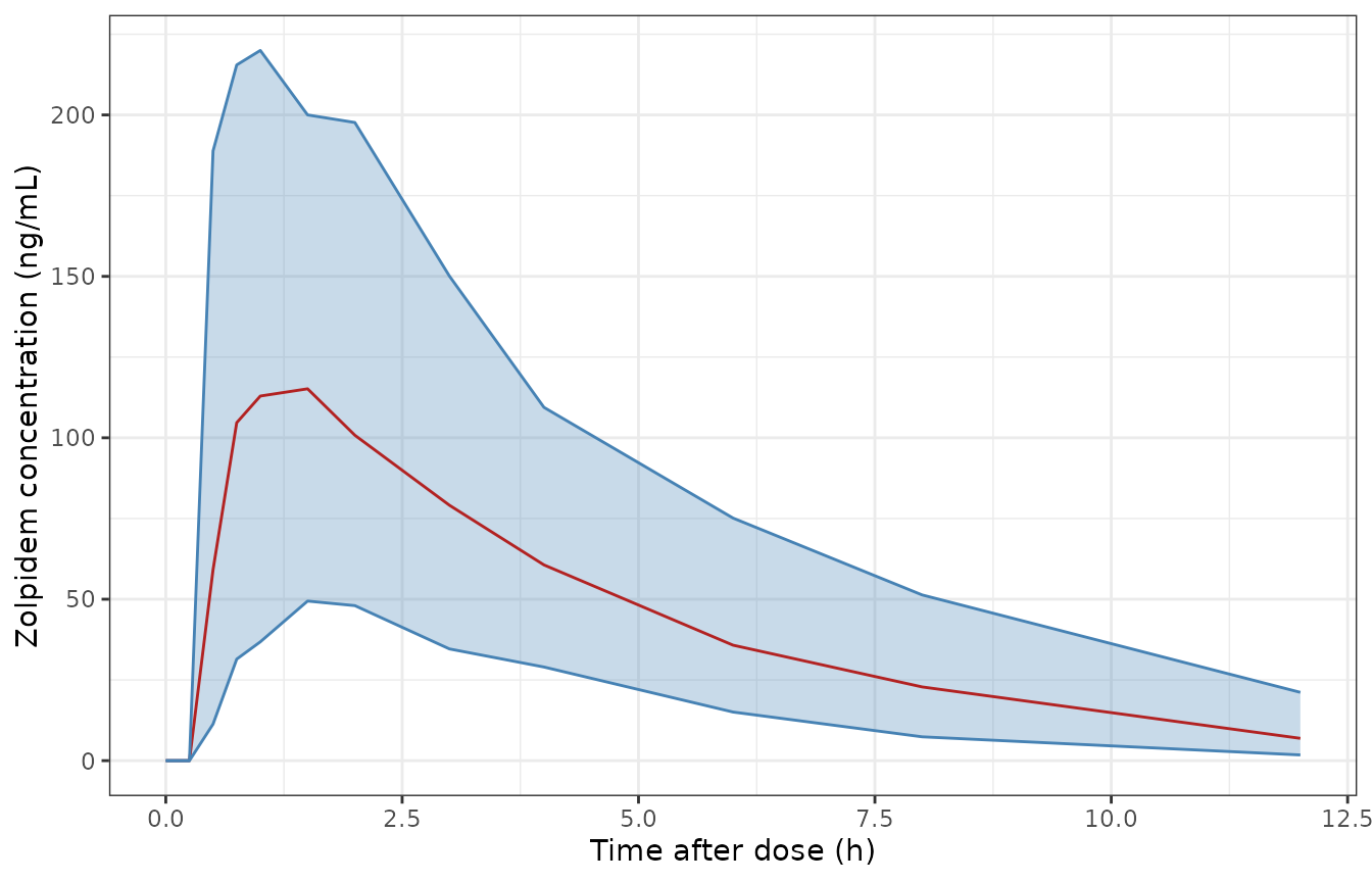
Replicates Figure 3 of Cha 2024: 5th, 50th and 95th percentiles of simulated observations (with residual error) after a single 10 mg dose, 200 subjects.
Figure 5 and Table 3: overdose simulations
Figure 5 and Table 3 simulate single oral doses of 10, 280, 560 and 1120 mg (one tablet, and one, two and four 28-tablet packages) without residual error. The paper used 500 subjects per dose; 200 are used here.
doses <- c(10, 280, 560, 1120)
n_arm <- 200
grid <- seq(0, 24, by = 0.05)
ev_od <- lapply(seq_along(doses), function(i) {
  rxode2::et(amt = doses[[i]], cmt = "depot") |>
    rxode2::et(grid, cmt = "central") |>
    rxode2::et(id = (i - 1) * n_arm + seq_len(n_arm)) |>
    as.data.frame() |>
    dplyr::mutate(dose_mg = doses[[i]])
}) |>
  dplyr::bind_rows()
rxode2::rxSetSeed(560)
sim_od <- rxode2::rxSolve(mod, events = ev_od, keep = "dose_mg", returnType = "data.frame")
thr <- data.frame(y = c(500, 1500, 4000), level = c("toxic", "comatose", "fatal"))
ggplot(sim_od, aes(time, Cc, group = id)) +
  geom_line(alpha = 0.15) +
  geom_hline(data = thr, aes(yintercept = y, colour = level)) +
  scale_colour_manual(values = c(toxic = "gold", comatose = "orange", fatal = "red")) +
  facet_wrap(~ paste(dose_mg, "mg"), scales = "free_y") +
  labs(x = "Time (h)", y = "Zolpidem concentration (ng/mL)", colour = NULL) +
  theme_bw()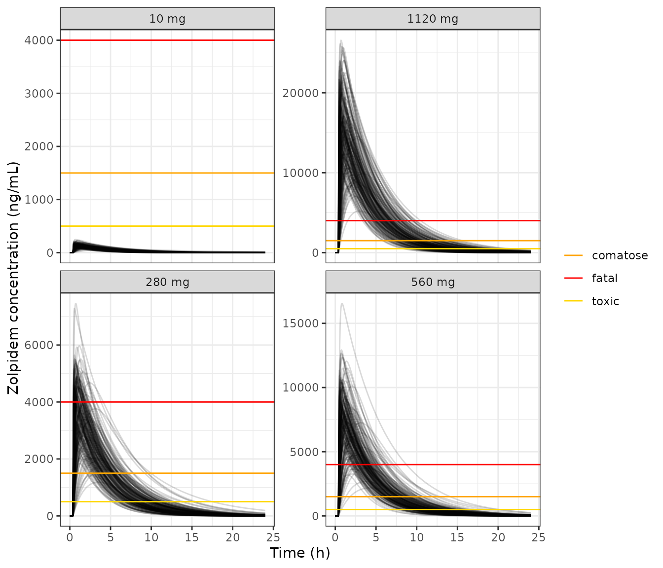
Replicates Figure 5 of Cha 2024: individual simulated profiles; yellow, orange and red lines mark the toxic (500), comatose (1500) and fatal (4000 ng/mL) thresholds.
Table 3 counts, per subject, the time the concentration stays above each threshold. Its “toxic” row is 100% “> 3 h” at every overdose; the time spent within the 500-1500 ng/mL band would put a few percent of the 280 mg subjects in the 2-3 h category, so the rows are read as cumulative time above 500, 1500 and 4000 ng/mL.
dt <- 0.05
dur_tab <- sim_od |>
  dplyr::group_by(dose_mg, id) |>
  dplyr::summarise(
    toxic = sum(Cc > 500) * dt, comatose = sum(Cc > 1500) * dt, fatal = sum(Cc > 4000) * dt,
    .groups = "drop"
  ) |>
  tidyr::pivot_longer(c(toxic, comatose, fatal), names_to = "level", values_to = "dur") |>
  dplyr::mutate(cat = cut(dur, c(-Inf, 0, 1, 2, 3, Inf), labels = c("NR", "<1 h", "1-2 h", "2-3 h", ">3 h"))) |>
  dplyr::count(level, dose_mg, cat, .drop = FALSE) |>
  dplyr::group_by(level, dose_mg) |>
  dplyr::mutate(pct = 100 * n / sum(n)) |>
  dplyr::ungroup()

paper_t3 <- tibble::tribble(
  ~level, ~dose_mg, ~NR, ~`<1 h`, ~`1-2 h`, ~`2-3 h`, ~`>3 h`,
  "toxic", 10, 100, 0, 0, 0, 0,
  "toxic", 280, 0, 0, 0, 0, 100,
  "toxic", 560, 0, 0, 0, 0, 100,
  "toxic", 1120, 0, 0, 0, 0, 100,
  "comatose", 10, 100, 0, 0, 0, 0,
  "comatose", 280, 0.2, 0.4, 0.8, 15.0, 83.6,
  "comatose", 560, 0, 0, 0, 0.4, 99.6,
  "comatose", 1120, 0, 0, 0, 0, 100,
  "fatal", 10, 100, 0, 0, 0, 0,
  "fatal", 280, 58.8, 21.4, 15.6, 4.0, 0.2,
  "fatal", 560, 2.6, 1.6, 11.2, 31.4, 53.2,
  "fatal", 1120, 0, 0, 0, 1.6, 98.4
) |>
  tidyr::pivot_longer(-c(level, dose_mg), names_to = "cat", values_to = "paper")

t3 <- dur_tab |>
  dplyr::mutate(cat = as.character(cat)) |>
  dplyr::left_join(paper_t3, by = c("level", "dose_mg", "cat"))
stopifnot(nrow(t3) == 60, !anyNA(t3$paper))

t3 |>
  dplyr::mutate(cell = sprintf("%.1f (%.1f)", pct, paper)) |>
  dplyr::select(level, dose_mg, cat, cell) |>
  tidyr::pivot_wider(names_from = cat, values_from = cell) |>
  dplyr::mutate(level = factor(level, c("toxic", "comatose", "fatal"))) |>
  dplyr::arrange(level, dose_mg) |>
  dplyr::rename(Threshold = level, `Dose (mg)` = dose_mg) |>
knitr::kable(caption = "Percent of subjects by time above each threshold: simulated, 200 per dose (Cha 2024 Table 3, 500 per dose, in parentheses).")| Threshold | Dose (mg) | NR | <1 h | 1-2 h | 2-3 h | >3 h |
|---|---|---|---|---|---|---|
| toxic | 10 | 100.0 (100.0) | 0.0 (0.0) | 0.0 (0.0) | 0.0 (0.0) | 0.0 (0.0) |
| toxic | 280 | 0.0 (0.0) | 0.0 (0.0) | 0.0 (0.0) | 0.0 (0.0) | 100.0 (100.0) |
| toxic | 560 | 0.0 (0.0) | 0.0 (0.0) | 0.0 (0.0) | 0.0 (0.0) | 100.0 (100.0) |
| toxic | 1120 | 0.0 (0.0) | 0.0 (0.0) | 0.0 (0.0) | 0.0 (0.0) | 100.0 (100.0) |
| comatose | 10 | 100.0 (100.0) | 0.0 (0.0) | 0.0 (0.0) | 0.0 (0.0) | 0.0 (0.0) |
| comatose | 280 | 1.0 (0.2) | 0.0 (0.4) | 3.5 (0.8) | 14.0 (15.0) | 81.5 (83.6) |
| comatose | 560 | 0.0 (0.0) | 0.0 (0.0) | 0.0 (0.0) | 0.0 (0.4) | 100.0 (99.6) |
| comatose | 1120 | 0.0 (0.0) | 0.0 (0.0) | 0.0 (0.0) | 0.0 (0.0) | 100.0 (100.0) |
| fatal | 10 | 100.0 (100.0) | 0.0 (0.0) | 0.0 (0.0) | 0.0 (0.0) | 0.0 (0.0) |
| fatal | 280 | 60.0 (58.8) | 18.0 (21.4) | 18.0 (15.6) | 3.5 (4.0) | 0.5 (0.2) |
| fatal | 560 | 4.0 (2.6) | 2.0 (1.6) | 14.0 (11.2) | 26.5 (31.4) | 53.5 (53.2) |
| fatal | 1120 | 0.0 (0.0) | 0.0 (0.0) | 0.0 (0.0) | 1.0 (1.6) | 99.0 (98.4) |
# Model-true cell values (4000-subject closed form above): fatal NR at 280 mg
# ~60%, fatal >3 h at 560 mg ~52%. The binomial SE at 200 subjects is <= 3.6
# points, so 15 points is > 4 SE yet still breaks on a mis-transcribed CL, V
# or ka, each of which moves these cells by tens of points.
cell <- function(lv, d, ct) {
  v <- t3$pct[t3$level == lv & t3$dose_mg == d & t3$cat == ct]
  if (length(v) != 1L) stop("no unique cell for ", lv, " ", d, " ", ct)
  v
}
stopifnot(
  abs(cell("fatal", 280, "NR") - 58.8) < 15,
  abs(cell("fatal", 560, ">3 h") - 53.2) < 15,
  cell("fatal", 1120, ">3 h") > 85,
  cell("comatose", 560, ">3 h") > 90,
  # A 10 mg dose stays below the toxic threshold (model 95th-percentile Cmax
  # ~200 ng/mL); a tolerance, not exact zero.
  cell("toxic", 10, "NR") > 98
)
Figure 4: the web application’s 200 mg example
ev_200 <- rxode2::et(amt = 200, cmt = "depot") |>
  rxode2::et(grid, cmt = "central") |>
  rxode2::et(id = seq_len(n_arm))
rxode2::rxSetSeed(200)
sim_200 <- rxode2::rxSolve(mod, events = ev_200, returnType = "data.frame")
band_200 <- sim_200 |>
  dplyr::group_by(time) |>
  dplyr::summarise(p05 = quantile(Cc, 0.05), p50 = median(Cc), p95 = quantile(Cc, 0.95), .groups = "drop")
ggplot(band_200, aes(time)) +
  geom_ribbon(aes(ymin = p05, ymax = p95), fill = "lightblue") +
  geom_line(aes(y = p50), colour = "steelblue4") +
  geom_hline(yintercept = c(200, 500, 1500, 4000), colour = c("grey50", "gold", "orange", "red")) +
  labs(x = "Time (h)", y = "Zolpidem concentration (ng/mL)") +
  theme_bw()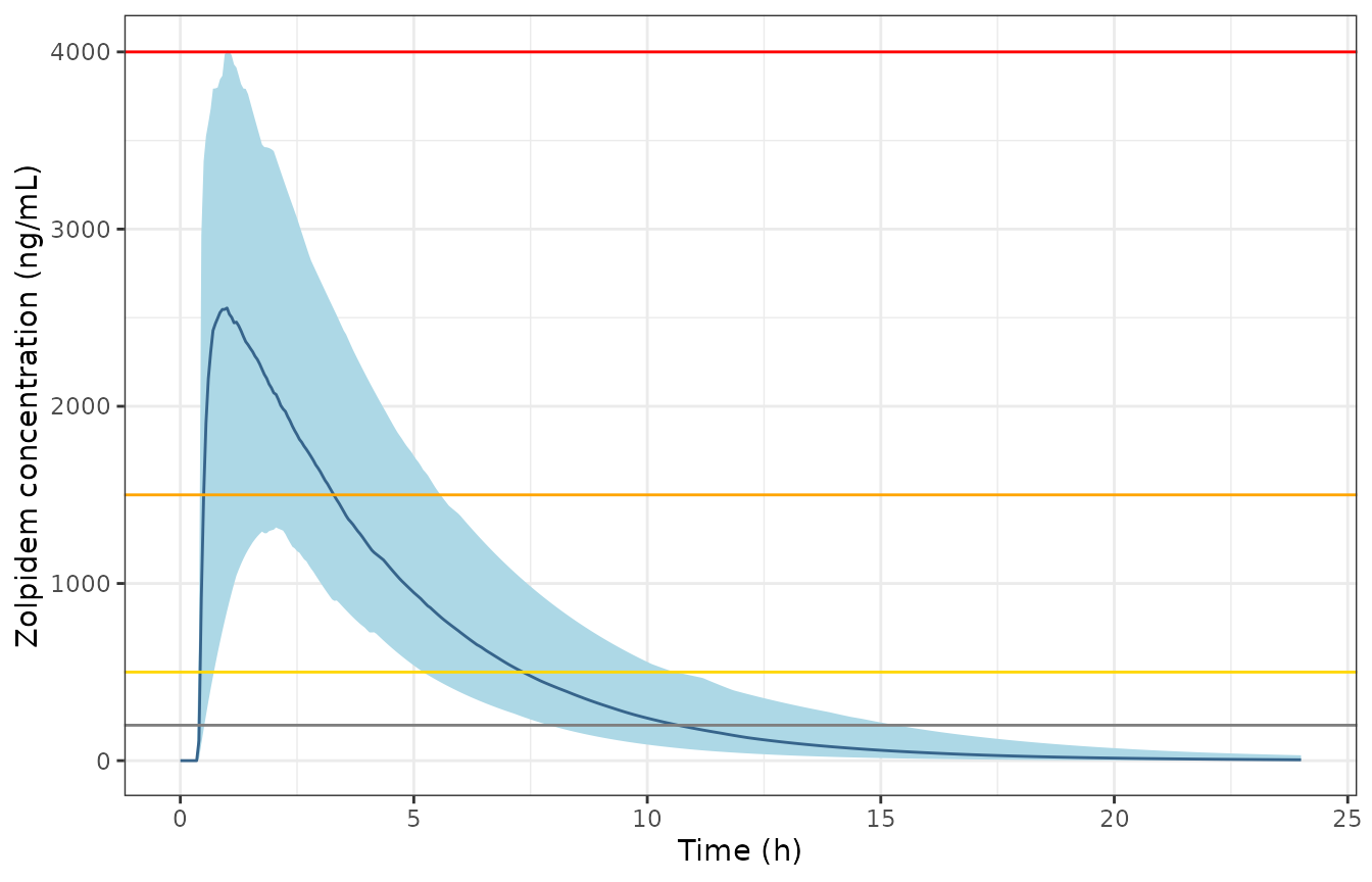
Replicates the simulation plot of Figure 4 of Cha 2024: 200 mg (twenty 10 mg tablets), median and 5th-95th percentile band of 200 simulated subjects.
The application’s panel reports a median concentration peaking near 2500 ng/mL with a 95th percentile just under 4000 ng/mL and a typical elimination rate constant of 0.27 1/h; the simulation above has the same shape and scale.
Assumptions and deviations
-
IIV scale. Table 2 prints the IIV rows as CV%. They
are encoded as
omega^2 = log(1 + CV^2), the reading that reproduces the paper’s Table 3 Monte Carlo summary;CV% = 100 * omegawould give twice the Ka variance and is inconsistent with Table 3 (see “Which scale did Table 2 use?”). -
Residual-error scale.
Proportional error 0.284is encoded as the SD of the proportional error; the variance reading would widen the simulated spread of the terminal slope beyond the digitised data. - Vd-CL correlation. Printed as a correlation (rho = 0.853) and converted to the covariance with the encoded variances.
- Terminal half-life. The model’s half-life (2.5 h typical) is shorter than the digitised NCA half-life (3.3 h); the model is used as published and this is not adjusted (see the NCA section).
- Table 3 thresholds. Read as cumulative time above 500, 1500 and 4000 ng/mL, the reading consistent with the printed 100% “> 3 h” toxic rows.
- Source data. The model was fitted to concentrations digitised from figures, not to the original measurements; the authors show the digitised NCA matches the original NCA (Table 1). No errata were found for the article (checked 2026-10-30).
- Dose in overdose. As the authors note, absorption after dozens of tablets may be slower or less complete than after one; the model carries the single-tablet absorption to all doses, as the paper’s simulations do.