Pinatuzumab vedotin + polatuzumab vedotin integrated two-analyte ADC PK (Lu 2016)
Source:vignettes/articles/Lu_2016_pinatuzumab_polatuzumab.Rmd
Lu_2016_pinatuzumab_polatuzumab.RmdModel and source
mod <- rxode2::rxode2(readModelDb("Lu_2016_pinatuzumab_polatuzumab"))
#> ℹ parameter labels from comments will be replaced by 'label()'- Citation: Lu D, Gibiansky L, Agarwal P, Dere RC, Li C, Chu Y-W, Hirata J, Joshi A, Jin JY, Girish S. Integrated Two-Analyte Population Pharmacokinetic Model for Antibody-Drug Conjugates in Patients: Implications for Reducing Pharmacokinetic Sampling. CPT Pharmacometrics Syst Pharmacol. 2016;5(12):665-673. doi:10.1002/psp4.12137
- Article: https://doi.org/10.1002/psp4.12137
- Supplement S1 (NONMEM control stream of Model 1), Supplemental Table 1 (study designs and sampling schemes): distributed with the article on the CPT:PSP site and with the open-access record PMC5192970.
Lu 2016 develops a single integrated population PK model that describes two analytes measured after administration of a monomethyl-auristatin-E (MMAE) antibody-drug conjugate (ADC):
- Tab – total antibody, i.e. the sum of fully conjugated, partially deconjugated and fully deconjugated antibody, measured in serum by ELISA.
- acMMAE – antibody-conjugated MMAE, the conjugate, measured in plasma by protein-A capture followed by LC-MS/MS and reported as MMAE equivalents.
Each analyte is a linear two-compartment system, and the two systems
share every parameter. The only structural difference is that acMMAE
carries an additional first-order deconjugation loss kdec
out of its central compartment: deconjugation destroys conjugate but not
antibody. That single asymmetry is what makes Tab predictable from
acMMAE and is the whole point of the paper – once kdec has
been estimated from intensively sampled phase I data, late-phase trials
can reduce or eliminate Tab sampling entirely.
Two ADCs sharing the same MC-VC-PABC linker and the same payload were
fitted jointly in one run: pinatuzumab vedotin
(anti-CD22) and polatuzumab vedotin (anti-CD79b). A molecule indicator
selects drug-specific values of CL, Vc, kdec and the acMMAE
assay cross-calibration slope; Q, Vp, all five IIV variances and both
residual errors are common to the two drugs. Following the policy of
building models as their authors built them, one jointly fitted model is
extracted as one model file, with the molecule indicator carried as the
mutually exclusive covariate pair TRT_PINATUZUMAB_VEDOTIN /
TRT_POLATUZUMAB_VEDOTIN.
cat(strwrap(mod$description, width = 78), sep = "\n")
#> Integrated two-analyte population PK model for the MMAE antibody-drug
#> conjugates pinatuzumab vedotin and polatuzumab vedotin in patients with
#> relapsed/refractory B-cell non-Hodgkin lymphoma (Lu 2016).
#> Antibody-conjugated MMAE (acMMAE; output Cc) and total antibody (Tab; output
#> Cc_tab) are each described by a linear two-compartment model that shares CL,
#> Q, Vc, Vp and all random effects, the only structural difference being an
#> additional first-order deconjugation loss kdec from the acMMAE central
#> compartment. The two ADCs are fitted jointly in one run: CL, Vc, kdec and the
#> acMMAE assay cross-calibration slope take molecule-specific values selected
#> by the TRT_PINATUZUMAB_VEDOTIN / TRT_POLATUZUMAB_VEDOTIN indicators, while Q,
#> Vp, the IIV and the residual errors are shared. States hold molar amounts
#> (nmol); the two observables are returned in ng/mL using the molecular weights
#> carried in the published control stream. No covariates were assessed.
#> Simulation requires dosing central and central_tab simultaneously with the
#> same molar antibody amount; f(central) applies the mean drug-to-antibody
#> ratio of 3.585.
Population
pop <- readModelDb("Lu_2016_pinatuzumab_polatuzumab")()$population
str(pop, max.level = 1)
#> List of 9
#>  $ species      : chr "human"
#>  $ n_subjects   : num 154
#>  $ n_studies    : num 2
#>  $ disease_state: chr "Relapsed or refractory B-cell non-Hodgkin's lymphoma; patients with chronic lymphocytic leukaemia were excluded"| __truncated__
#>  $ dose_range   : chr "Pinatuzumab vedotin 0.1 to 3.2 mg/kg Q3W (dose expansion at 2.4 mg/kg) and polatuzumab vedotin 0.1 to 2.4 mg/kg"| __truncated__
#>  $ studies      : chr "Dataset 1 (the phase I development dataset behind Model 1) pooled DCT4862g (NCT01209130, pinatuzumab vedotin: 6"| __truncated__
#>  $ covariates   : chr "None. Lu 2016 states that a relatively simple model without covariates was preferred given the goals of the ana"| __truncated__
#>  $ notes        : chr "Both ADCs link monomethyl auristatin E to the antibody through the same protease-labile MC-VC-PABC linker and s"| __truncated__
#>  $ dosing_note  : chr "Each ADC administration generates input to BOTH analytes. To simulate, provide TWO dose events per administrati"| __truncated__
The model file carries the estimates of Model 1, the fit to dataset 1 (the phase I development dataset). Per Lu 2016 Supplemental Table 1 that dataset pooled 154 patients with relapsed or refractory B-cell non-Hodgkin’s lymphoma across two phase I studies: DCT4862g (NCT01209130, pinatuzumab vedotin, 65 single-agent plus 15 rituximab-combination subjects, 0.1 to 3.2 mg/kg Q3W with dose expansion at 2.4 mg/kg) and DCS4968g (NCT01290549, polatuzumab vedotin, 66 single-agent plus 8 rituximab-combination subjects, 0.1 to 2.4 mg/kg Q3W with dose expansion at 2.4 mg/kg). Patients with chronic lymphocytic leukaemia were excluded. Sampling was intensive, more than 35 serum and plasma samples per patient in the single-agent cohorts.
Lu 2016 deliberately fitted no covariates: “Given these major goals, a relatively simple population pharmacokinetic model without covariates is more desirable, thus the covariate assessment was not performed.” The only subject-level classifier in the model is therefore which ADC the patient received. Baseline demographics are not tabulated in the article, and in particular body weight is not reported, which matters for the exposure comparison below.
Source trace
Every ini() value and every model()
equation, with its location in the source. “Table 1 / Model 1” is the
first numeric column pair of Lu 2016 Table 1, the fit to the phase I
dataset.
| Model element | Value | Source |
|---|---|---|
lcl_pina |
log(0.0292) L/h | Table 1, row “Pinatuzumab vedotin clearance: CLpina (L/hr)”, Model 1 |
lcl_pola |
log(0.0355) L/h | Table 1, row “Polatuzumab vedotin clearance: CLpola (L/hr)”, Model 1 |
lq |
log(0.0267) L/h | Table 1, row “Intercompartment clearance: Q (L/hr)”, Model 1 |
lvc_pina |
log(5.35) L | Table 1, row “Pinatuzumab vedotin central volume: VC,pina (L)”, Model 1 |
lvc_pola |
log(5.00) L | Table 1, row “Polatuzumab vedotin central volume: VC,pola (L)”, Model 1 |
lvp |
log(8.21) L | Table 1, row “Peripheral volume: VP (L)”, Model 1 |
lkdec_pina |
log(0.00855) 1/h | Table 1, row “Pinatuzumab vedotin deconjugation rate: kdec,pina (1/hr)”, Model 1 |
lkdec_pola |
log(0.00647) 1/h | Table 1, row “Polatuzumab vedotin deconjugation rate: kdec,pola (1/hr)”, Model 1 |
cal_slope_acmmae_pina |
1.31 | Table 1, row “Pinatuzumab vedotin assay correction: CORRpina”, Model 1; Eq. 5 |
cal_slope_acmmae_pola |
1.45 | Table 1, row “Polatuzumab vedotin assay correction: CORRpola”, Model 1; Eq. 5 |
etalcl |
0.488 | Table 1, row “Random effect on CL: omega^2 CL”, Model 1 (a variance) |
etalq |
0.269 | Table 1, row “Random effect on Q: omega^2 Q”, Model 1 |
etalvc |
0.0519 | Table 1, row “Random effect on VC: omega^2 VC”, Model 1 |
etalvp |
0.707 | Table 1, row “Random effect on VP: omega^2 VP”, Model 1 |
etalkdec |
0.053 | Table 1, row “Random effect on kdec: omega^2 kdec”, Model 1 |
propSd |
sqrt(0.0314) = 0.17720 | Table 1, row “Residual error for acMMAE: sigma^2 acMMAE”, Model 1;
form from supplement S1 $ERROR
|
propSd_tab |
sqrt(0.0585) = 0.241868 | Table 1, row “Residual error for Tab: sigma^2 Tab”, Model 1; form
from supplement S1 $ERROR
|
mdar = 3.585 |
unitless | Figure 2 legend and Methods: mean drug-to-antibody ratio of the dosing solution measured by HIC, identical for both ADCs |
mw_tab = 146.455 |
(ng/mL) per (nmol/L) | Supplement S1 $ERROR:
coDose = 146455/1000
|
mw_mmae = 0.718 |
(ng/mL) per (nmol/L) | Supplement S1 $ERROR:
ACMMAE = A(3)/V1*0.718
|
d/dt(central_tab) |
-(kel + k12) * central_tab + k21 * peripheral1_tab |
Eq. 1 (supplement S1 $DES DADT(1), commented “Tab
CENTRAL”) |
d/dt(peripheral1_tab) |
k12 * central_tab - k21 * peripheral1_tab |
Eq. 2 ($DES DADT(2)) |
d/dt(central) |
-(kel + k12) * central - kdec * central + k21 * peripheral1 |
Eq. 3 ($DES DADT(3), commented “acMMAE CENTRAL”) |
d/dt(peripheral1) |
k12 * central - k21 * peripheral1 |
Eq. 4 ($DES DADT(4)) |
kel = cl/vc, k12 = q/vc,
k21 = q/vp
|
– | Text following Eq. 4 and Figure 2 legend; supplement S1
$PK
|
f(central) <- mdar |
– | Figure 2 legend initial conditions: A1(0) = DTab, A3(0) = DacMMAE = mDAR * DTab |
| molecule selection | lcl_pina * TRT_PINATUZUMAB_VEDOTIN + lcl_pola * TRT_POLATUZUMAB_VEDOTIN |
Supplement S1 $PK:
CL = (THETA(1)*(2-MOL)+THETA(7)*(MOL-1))*EXP(ETA(1)),
likewise V1, KDEC, CORR |
Cc <- corr * mw_mmae * central / vc |
– | Eq. 5 with supplement S1 $ERROR:
ACMMAE = A(3)/V1*0.718,
IF (TYPE.EQ.2) TY = CORR*ACMMAE
|
Cc_tab <- mw_tab * central_tab / vc |
– | Supplement S1 $ERROR:
TA = coDose*A(1)/V1
|
Cc ~ prop(propSd),
Cc_tab ~ prop(propSd_tab)
|
– | Supplement S1 $ERROR: Y = TY*(1+EPS(n)),
proportional in linear space |
Two readings that the supplement settles and that the article alone leaves open are recorded here because they change the numbers:
-
The Table 1 random-effect and residual entries are
variances, not standard deviations. The column headings are
omega^2andsigma^2, the supplement S1$OMEGAblock specifies the same quantities on the NONMEM variance scale with initial values (0.43, 0.18, 0.05, 0.58, 0.03) that bracket the reported finals, and the reported RSE of 13.2% onomega^2 CLmatches thesqrt(2/n)= 11.4% expected for a variance at n = 154 rather than the ~5.7% expected for a standard deviation. Read as standard deviations the residual errors would be 5.9% and 5.6%, which no patient-sample ELISA or LC-MS/MS assay achieves. -
The residual error is proportional in linear space,
not log-additive or exponential:
$ERRORcomputesY = TY*(1+EPS(1))andY = TY*(1+EPS(2)).
Internal consistency of the transcribed Table 1 values
Lu 2016 Results states: “Differences in CL, VC, kdec, and CORR parameters for pinatuzumab vedotin and polatuzumab vedotin were 18%, 7%, 32%, and 10%, respectively.” That sentence is an arithmetic check on exactly the four molecule-specific parameter pairs this file carries, so it confirms the correct Table 1 column was transcribed.
theta <- function(nm) exp(mod$theta[[nm]])
bare <- function(nm) mod$theta[[nm]]

pairs_chk <- tibble::tibble(
  parameter = c("CL", "VC", "kdec", "CORR"),
  pina = c(theta("lcl_pina"), theta("lvc_pina"), theta("lkdec_pina"), bare("cal_slope_acmmae_pina")),
  pola = c(theta("lcl_pola"), theta("lvc_pola"), theta("lkdec_pola"), bare("cal_slope_acmmae_pola")),
  published_pct = c(18, 7, 32, 10)
) |>
  dplyr::mutate(
    # The paper does not say which value is the denominator; report both and
    # keep the closer one, which is what a relative difference of a pair means.
    pct_a = 100 * abs(pina - pola) / pmax(pina, pola),
    pct_b = 100 * abs(pina - pola) / pmin(pina, pola),
    best_pct = ifelse(
      abs(pct_a - published_pct) < abs(pct_b - published_pct), pct_a, pct_b
    ),
    abs_error_pp = abs(best_pct - published_pct)
  )

knitr::kable(
  pairs_chk |>
    dplyr::select(
      "Parameter" = parameter, "Pinatuzumab vedotin" = pina,
      "Polatuzumab vedotin" = pola, "Difference (%)" = best_pct,
      "Published (%)" = published_pct
    ),
  digits = c(0, 5, 5, 1, 0),
  caption = "Reproduces the CL / VC / kdec / CORR difference sentence in Lu 2016 Results."
)| Parameter | Pinatuzumab vedotin | Polatuzumab vedotin | Difference (%) | Published (%) |
|---|---|---|---|---|
| CL | 0.02920 | 0.03550 | 17.7 | 18 |
| VC | 5.35000 | 5.00000 | 7.0 | 7 |
| kdec | 0.00855 | 0.00647 | 32.1 | 32 |
| CORR | 1.31000 | 1.45000 | 9.7 | 10 |
Every one of the four reproduces the published percentage to within one percentage point, so the Model 1 column was read correctly.
Virtual cohort
There are no covariates to sample. The cohort varies only through the five random effects, and is split into two equally sized arms, one per ADC, using common random numbers so the two drugs are compared on matched subjects.
Doses are expressed in the model’s molar unit (nmol of antibody).
Converting the clinical 2.4 mg/kg Q3W regimen needs a body weight,
which Lu 2016 does not report. The sibling model
Lu_2019_polatuzumab (same first author, same drug,
overlapping NHL programme) uses 75 kg as its weight-normalisation
reference, so 75 kg is adopted here and flagged in the Errata as an
assumption that is not paper-derived.
nSubPerArm <- 100L
wtKg <- 75 # ASSUMPTION, not from Lu 2016; see Errata
mwAdc <- 146455 # g/mol, supplement S1 $ERROR coDose
doseMgPerKg <- 2.4
doseNmol <- doseMgPerKg * wtKg * 1e6 / mwAdc

tau <- 504 # h, Q3W
nCycles <- 40L
tLastDose <- tau * (nCycles - 1L)

doseNmol
#> [1] 1229.046
Forty Q3W cycles are simulated so that the last dosing interval is at
true steady state for essentially every subject. The Tab terminal
half-life implied by the Model 1 typical parameters is about 480 h, so
twelve cycles would be ample for a typical subject – but with
omega^2 of 0.488 on CL and 0.707 on Vp, a subject drawn at
the slow end of both distributions has a terminal half-life several
times that and is still accumulating. Lu 2016 computed its Table 2
exposures “using individual post-hoc PK parameters and the analytical
solution for a two-compartment model”, i.e. exactly at steady state, so
the simulation has to get there too before the comparison is fair. Forty
cycles is a numerical device, not a clinical regimen; nothing in the
model is time-dependent, so it does not change the steady state
itself.
obsRelLast <- sort(unique(c(seq(0, 24, by = 0.5), seq(24, tau, by = 4))))
obsRelFirst <- sort(unique(c(seq(0, 24, by = 1), seq(24, tau, by = 12))))

makeArm <- function(idStart, nSub, pina,
                    times = c(obsRelFirst, tLastDose + obsRelLast),
                    addl = nCycles - 1L) {
  ids <- seq.int(idStart, idStart + nSub - 1L)
  dose <- expand.grid(
    id = ids,
    cmt = c("central_tab", "central"),
    stringsAsFactors = FALSE
  )
  dose$time <- 0
  dose$amt <- doseNmol
  dose$evid <- 1L
  dose$ii <- tau
  dose$addl <- addl
  dose$dvid <- 0L

  obs <- expand.grid(
    id = ids,
    time = times,
    stringsAsFactors = FALSE
  )
  obs$cmt <- "central"
  obs$amt <- 0
  obs$evid <- 0L
  obs$ii <- 0
  obs$addl <- 0L
  obs$dvid <- 1L

  keepCols <- c("id", "time", "amt", "evid", "cmt", "ii", "addl", "dvid")
  out <- rbind(dose[, keepCols], obs[, keepCols])
  out$TRT_PINATUZUMAB_VEDOTIN <- as.integer(pina)
  out$TRT_POLATUZUMAB_VEDOTIN <- as.integer(!pina)
  out$treatment <- if (pina) "Pinatuzumab vedotin" else "Polatuzumab vedotin"
  out[order(out$id, out$time, -out$evid), ]
}

evPina <- makeArm(1L, nSubPerArm, pina = TRUE)
evPola <- makeArm(1000L + 1L, nSubPerArm, pina = FALSE)
nrow(evPina) + nrow(evPola)
#> [1] 47200
Simulation
Each ADC administration produces input to both analytes. Two dose
records are supplied per administration – one into
central_tab and one into central – carrying
the same molar antibody amount; the model’s
f(central) <- mdar scales the acMMAE input to
mDAR * DTab, reproducing the Lu 2016 Figure 2 initial
conditions.
Observation rows sit on the ODE state
central and carry dvid = 1. The
dvid column is what a two-endpoint model needs in order to
accept an observation addressed to an ODE state rather than to an
endpoint: without it rxode2 rejects the record with
'dvid'->'cmt' or 'cmt' on observation record or on a undefined compartment.
Naming an algebraic observable on the record instead
(cmt = "Cc") also solves it, but addressing ODE states by
name keeps the event table honest about what is being sampled. Either
way rxSolve() returns both observables (Cc,
Cc_tab) and all four state amounts as columns on every
observation row.
rxode2::rxSetSeed(20161110)
simPina <- rxode2::rxSolve(mod, evPina, addDosing = FALSE, keep = "treatment")

rxode2::rxSetSeed(20161110) # common random numbers across the two arms
simPola <- rxode2::rxSolve(mod, evPola, addDosing = FALSE, keep = "treatment")

sim <- dplyr::bind_rows(
  tibble::as_tibble(simPina),
  tibble::as_tibble(simPola)
)
dplyr::glimpse(sim[, c("id", "time", "treatment", "Cc", "Cc_tab", "cl", "vc", "kdec", "corr")])
#> Rows: 46,800
#> Columns: 9
#> $ id        <int> 1, 1, 1, 1, 1, 1, 1, 1, 1, 1, 1, 1, 1, 1, 1, 1, 1, 1, 1, 1, …
#> $ time      <dbl> 0, 1, 2, 3, 4, 5, 6, 7, 8, 9, 10, 11, 12, 13, 14, 15, 16, 17…
#> $ treatment <chr> "Pinatuzumab vedotin", "Pinatuzumab vedotin", "Pinatuzumab v…
#> $ Cc        <dbl> 504.2089, 497.1452, 490.1838, 483.3234, 476.5624, 469.8993, …
#> $ Cc_tab    <dbl> 21899.28, 21732.13, 21566.41, 21402.11, 21239.20, 21077.68, …
#> $ cl        <dbl> 0.04263457, 0.04263457, 0.04263457, 0.04263457, 0.04263457, …
#> $ vc        <dbl> 8.219449, 8.219449, 8.219449, 8.219449, 8.219449, 8.219449, …
#> $ kdec      <dbl> 0.006446854, 0.006446854, 0.006446854, 0.006446854, 0.006446…
#> $ corr      <dbl> 1.31, 1.31, 1.31, 1.31, 1.31, 1.31, 1.31, 1.31, 1.31, 1.31, …
Concentration-time profiles
Lu 2016 Supplemental Figure 3 shows a dose-normalised VPC of both analytes for both molecules. The equivalent simulated profiles over the first cycle are reproduced below; the observed data are not distributed with the article, so this replicates the simulated side of that figure only.
profile <- sim |>
  dplyr::filter(time <= tau) |>
  dplyr::select(id, time, treatment, Cc, Cc_tab) |>
  tidyr::pivot_longer(c(Cc, Cc_tab), names_to = "analyte", values_to = "conc") |>
  dplyr::mutate(
    analyte = dplyr::recode(analyte, Cc = "acMMAE (ng/mL)", Cc_tab = "Tab (ng/mL)")
  )

profileSummary <- profile |>
  dplyr::group_by(treatment, analyte, time) |>
  dplyr::summarise(
    p05 = quantile(conc, 0.05), p50 = median(conc), p95 = quantile(conc, 0.95),
    .groups = "drop"
  )

ggplot2::ggplot(profileSummary, ggplot2::aes(time / 24, p50)) +
  ggplot2::geom_ribbon(ggplot2::aes(ymin = p05, ymax = p95), alpha = 0.2) +
  ggplot2::geom_line() +
  ggplot2::facet_grid(analyte ~ treatment, scales = "free_y") +
  ggplot2::scale_y_log10() +
  ggplot2::labs(
    x = "Days after the first dose",
    y = "Concentration (ng/mL)",
    caption = "Median with 5th-95th percentile band, cycle 1, 2.4 mg/kg Q3W at an assumed 75 kg."
  ) +
  ggplot2::theme_bw()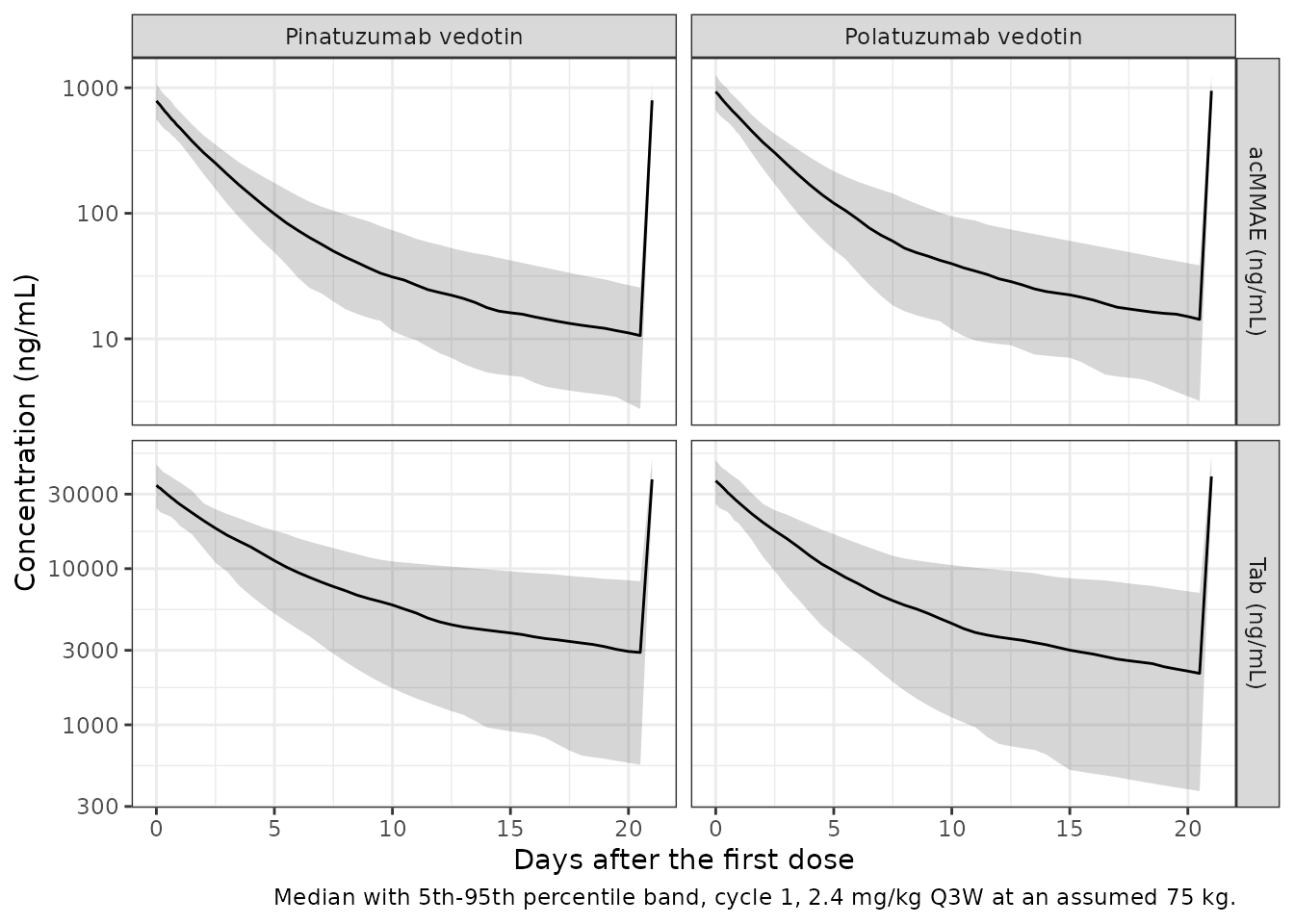
Average drug-to-antibody ratio declines with time
The mechanism the model encodes is that deconjugation converts
high-DAR species to low-DAR species, so the molar ratio of acMMAE to Tab
– the average DAR of the circulating conjugate – falls monotonically
from its value in the dosing solution. Because the assay
cross-calibration slope applies to the acMMAE observable, the ratio
computed from the two predicted observations starts at
corr * mdar, not at mdar; that is precisely
the systematic excess Lu 2016 measured at 0.5 h post end of infusion and
introduced CORR to absorb.
darDf <- sim |>
  dplyr::filter(time <= tau) |>
  dplyr::mutate(
    # back out molar concentrations from the two ng/mL observables
    dar_observed = (Cc / 0.718) / (Cc_tab / 146.455)
  )

darSummary <- darDf |>
  dplyr::group_by(treatment, time) |>
  dplyr::summarise(p50 = median(dar_observed), .groups = "drop")

ggplot2::ggplot(darSummary, ggplot2::aes(time / 24, p50, colour = treatment)) +
  ggplot2::geom_line(linewidth = 0.8) +
  ggplot2::geom_hline(yintercept = 3.585, linetype = "dashed") +
  ggplot2::labs(
    x = "Days after the first dose", y = "Molar acMMAE : Tab ratio",
    colour = NULL,
    caption = "Dashed line: mDAR = 3.585 measured in the dosing solution by HIC."
  ) +
  ggplot2::theme_bw() +
  ggplot2::theme(legend.position = "bottom")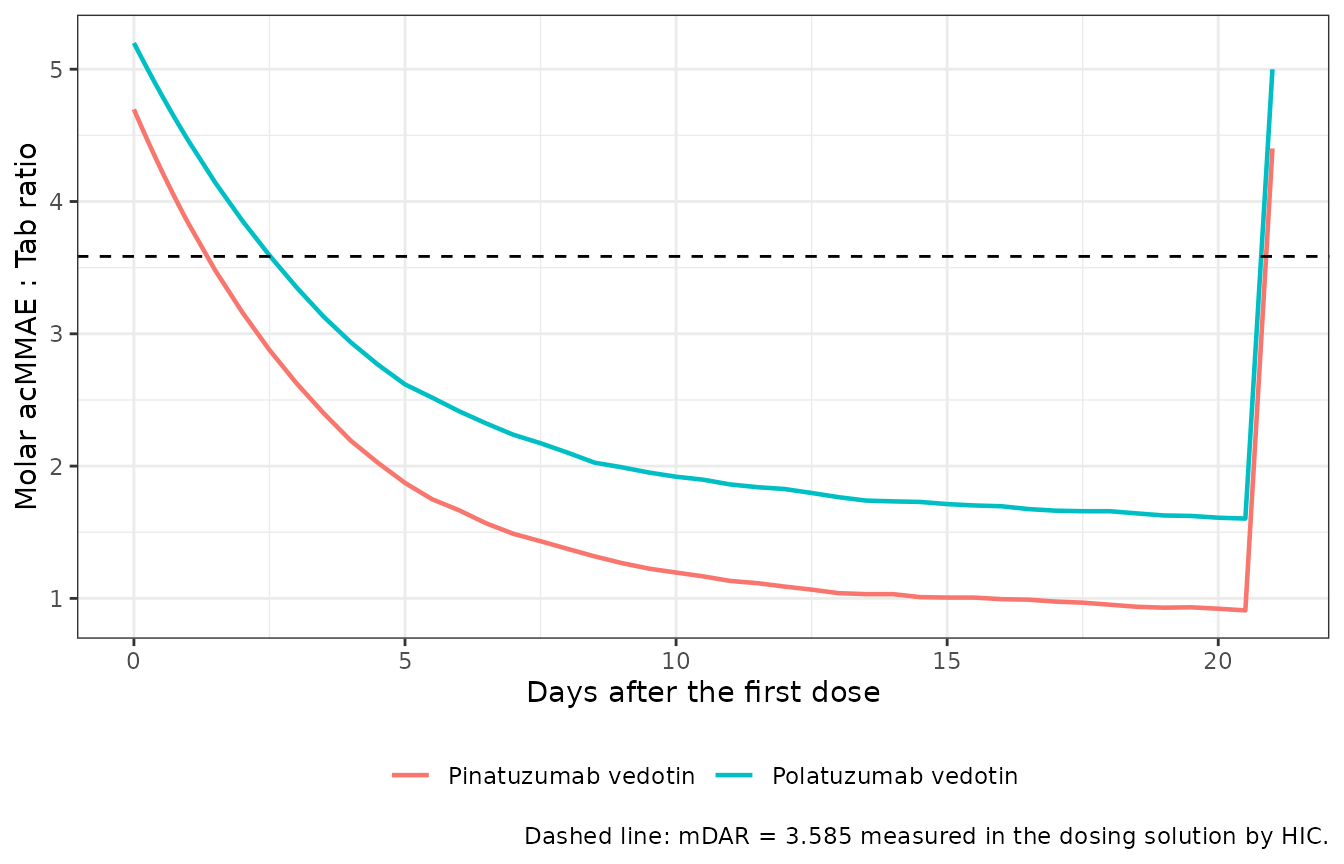
The zero-time intercept is an exact property of the encoding:
immediately after a dose the whole conjugate amount is
mdar * DTab and the whole antibody amount is
DTab, so the ratio of the two predicted observables must be
corr * mdar for every subject, independent of the random
effects.
intercept <- darDf |>
  dplyr::filter(time == 0) |>
  dplyr::group_by(treatment) |>
  dplyr::summarise(
    observed = median(dar_observed),
    expected = median(corr) * 3.585,
    .groups = "drop"
  ) |>
  dplyr::mutate(rel_error = abs(observed - expected) / expected)

knitr::kable(intercept, digits = c(0, 4, 4, 8))| treatment | observed | expected | rel_error |
|---|---|---|---|
| Pinatuzumab vedotin | 4.6964 | 4.6964 | 0 |
| Polatuzumab vedotin | 5.1983 | 5.1982 | 0 |
Closed-form validation
Both analytes are linear, so the steady-state exposure over one
dosing interval has an exact closed form that the numerical solution
must reproduce. These identities are strong structural checks: a dropped
kdec term, an f(central) that did not apply, a
wrong micro-constant or a mis-scaled observable all break them.
- Tab is eliminated only through
CL, so the interval exposure of the Tab observable ismw_tab * DTab / cl. - acMMAE carries an additional first-order loss
kdecfrom its central compartment, so its effective clearance iscl + kdec * vc, its dose ismdar * DTab, and its observable also carriescorr. The interval exposure is thereforecorr * mw_mmae * mdar * DTab / (cl + kdec * vc).
The sharpest form of the check is the mass-balance
identity, which holds exactly at every time point and so needs
neither steady state nor extrapolation to infinity. Integrating the
system over [0, T] after a single dose,
cl * AUC_molar_tab(0, T) = DTab - (central_tab(T) + peripheral1_tab(T))(cl + kdec * vc) * AUC_molar_acMMAE(0, T) = mdar * DTab - (central(T) + peripheral1(T))
Any deviation beyond trapezoidal error means the encoded ODEs do not conserve what they should. This is run on a dedicated single-dose solve over a dense grid, on the same subjects.
sdGrid <- sort(unique(c(seq(0, 24, by = 0.5), seq(24, 504, by = 4), seq(504, 2016, by = 24))))

rxode2::rxSetSeed(20161110)
sdPina <- rxode2::rxSolve(
  mod, makeArm(1L, nSubPerArm, pina = TRUE, times = sdGrid, addl = 0L),
  addDosing = FALSE, keep = "treatment"
)
rxode2::rxSetSeed(20161110)
sdPola <- rxode2::rxSolve(
  mod, makeArm(1000L + 1L, nSubPerArm, pina = FALSE, times = sdGrid, addl = 0L),
  addDosing = FALSE, keep = "treatment"
)
simSd <- dplyr::bind_rows(tibble::as_tibble(sdPina), tibble::as_tibble(sdPola))

trapz <- function(x, y) sum(diff(x) * (utils::head(y, -1) + utils::tail(y, -1)) / 2)

massBalance <- simSd |>
  dplyr::arrange(id, time) |>
  dplyr::group_by(id, treatment) |>
  dplyr::summarise(
    eliminated_tab = dplyr::first(cl) * trapz(time, Cc_tab) / 146.455,
    remaining_tab = doseNmol - (dplyr::last(central_tab) + dplyr::last(peripheral1_tab)),
    eliminated_acmmae = (dplyr::first(cl) + dplyr::first(kdec) * dplyr::first(vc)) *
      trapz(time, Cc) / (dplyr::first(corr) * 0.718),
    remaining_acmmae = 3.585 * doseNmol - (dplyr::last(central) + dplyr::last(peripheral1)),
    .groups = "drop"
  ) |>
  dplyr::mutate(
    err_tab = abs(eliminated_tab - remaining_tab) / remaining_tab,
    err_acmmae = abs(eliminated_acmmae - remaining_acmmae) / remaining_acmmae
  )

knitr::kable(
  massBalance |>
    dplyr::group_by(treatment) |>
    dplyr::summarise(
      "Median Tab error" = median(err_tab), "Max Tab error" = max(err_tab),
      "Median acMMAE error" = median(err_acmmae), "Max acMMAE error" = max(err_acmmae),
      .groups = "drop"
    ) |>
    dplyr::rename("Treatment" = treatment),
  digits = 7,
  caption = "Mass balance: cumulative elimination vs dose minus amount remaining at 2016 h."
)| Treatment | Median Tab error | Max Tab error | Median acMMAE error | Max acMMAE error |
|---|---|---|---|---|
| Pinatuzumab vedotin | 0.0000998 | 0.0003940 | 0.0002648 | 0.0006354 |
| Polatuzumab vedotin | 0.0001269 | 0.0005422 | 0.0002570 | 0.0007184 |
# Pure numerical error (trapezoidal quadrature), identical across machines, so a
# max() bound is the right assertion here rather than a robust quantile.
stopifnot(
  max(massBalance$err_tab) < 0.002,
  max(massBalance$err_acmmae) < 0.002
)
Mass balance closes to better than one part in a thousand for every
subject in both arms, for both analytes: the ODE encoding, the
f(central) dose scaling, the micro-constants and the
observable scalings are all mutually consistent.
The steady-state interval exposure is the same identity specialised to a repeated-dose regimen, and is the quantity Lu 2016 Table 2 reports.
closed <- sim |>
  dplyr::filter(time >= tLastDose) |>
  dplyr::arrange(id, time) |>
  dplyr::group_by(id, treatment) |>
  dplyr::summarise(
    auc_tab_sim = trapz(time, Cc_tab),
    auc_acmmae_sim = trapz(time, Cc),
    auc_tab_closed = 146.455 * doseNmol / dplyr::first(cl),
    auc_acmmae_closed = dplyr::first(corr) * 0.718 * 3.585 * doseNmol /
      (dplyr::first(cl) + dplyr::first(kdec) * dplyr::first(vc)),
    .groups = "drop"
  ) |>
  dplyr::mutate(
    err_tab = abs(auc_tab_sim - auc_tab_closed) / auc_tab_closed,
    err_acmmae = abs(auc_acmmae_sim - auc_acmmae_closed) / auc_acmmae_closed
  )

knitr::kable(
  closed |>
    dplyr::group_by(treatment) |>
    dplyr::summarise(
      "Median Tab error" = median(err_tab),
      "90th pctile Tab error" = quantile(err_tab, 0.9),
      "Median acMMAE error" = median(err_acmmae),
      "90th pctile acMMAE error" = quantile(err_acmmae, 0.9),
      .groups = "drop"
    ) |>
    dplyr::rename("Treatment" = treatment),
  digits = 5,
  caption = "Final-cycle interval exposure vs the steady-state closed form."
)| Treatment | Median Tab error | 90th pctile Tab error | Median acMMAE error | 90th pctile acMMAE error |
|---|---|---|---|---|
| Pinatuzumab vedotin | 7e-05 | 0.00017 | 0.00023 | 0.00035 |
| Polatuzumab vedotin | 9e-05 | 0.00022 | 0.00022 | 0.00037 |
# Robust quantile rather than max(): a handful of subjects drawn at the slow end
# of both the CL and the Vp distribution are still accumulating even after forty
# cycles, and which subjects those are is not reproducible across rxode2 builds.
stopifnot(
  quantile(closed$err_tab, 0.95) < 0.005,
  quantile(closed$err_acmmae, 0.95) < 0.005
)
Ninety-five percent of subjects reach the closed form to better than a tenth of a percent in both arms. The residual tail is the slow-disposition corner of the random-effect distribution described above, and it is a property of the model rather than a numerical artefact.
A second consequence worth stating explicitly, because it is the quantitative core of the paper: the ratio of the two effective clearances is what makes Tab recoverable from acMMAE.
sim |>
  dplyr::filter(time == 0) |>
  dplyr::group_by(treatment) |>
  dplyr::summarise(
    "Typical CL (L/h)" = median(cl),
    "Typical kdec * Vc (L/h)" = median(kdec * vc),
    "acMMAE effective CL / Tab CL" = median((cl + kdec * vc) / cl),
    .groups = "drop"
  ) |>
  dplyr::rename("Treatment" = treatment) |>
knitr::kable(digits = 4)| Treatment | Typical CL (L/h) | Typical kdec * Vc (L/h) | acMMAE effective CL / Tab CL |
|---|---|---|---|
| Pinatuzumab vedotin | 0.0266 | 0.0441 | 2.6255 |
| Polatuzumab vedotin | 0.0323 | 0.0312 | 1.9456 |
Deconjugation contributes roughly as much conjugate elimination as
proteolytic catabolism does, which is why acMMAE and Tab profiles
diverge steadily and why kdec is estimable with an RSE
below 5% from paired data.
PKNCA validation
Steady-state non-compartmental parameters over the final dosing interval, one set per analyte, grouped by treatment.
doseDf <- dplyr::bind_rows(evPina, evPola) |>
  dplyr::filter(evid == 1, cmt == "central_tab") |>
  dplyr::select(id, time, amt, treatment)

startSs <- tLastDose
endSs <- tLastDose + tau

ssIntervals <- data.frame(
  start = startSs,
  end = endSs,
  cmax = TRUE,
  tmax = TRUE,
  cmin = TRUE,
  auclast = TRUE,
  cav = TRUE
)
concTab <- sim |>
  dplyr::filter(!is.na(Cc_tab)) |>
  dplyr::transmute(id, time, Cc = Cc_tab, treatment)

ncaTab <- PKNCA::pk.nca(PKNCA::PKNCAdata(
  PKNCA::PKNCAconc(concTab, Cc ~ time | treatment + id,
                   concu = "ng/mL", timeu = "h"),
  PKNCA::PKNCAdose(doseDf, amt ~ time | treatment + id, doseu = "nmol"),
  intervals = ssIntervals
))
summary(ncaTab)
#>  Interval Start Interval End           treatment   N AUClast (h*ng/mL)
#>           19656        20160 Pinatuzumab vedotin 100     6.53e6 [59.9]
#>           19656        20160 Polatuzumab vedotin 100     5.37e6 [59.9]
#>  Cmax (ng/mL) Cmin (ng/mL)             Tmax (h)  Cav (ng/mL)
#>  41300 [23.8]   4950 [157] 0.000 [0.000, 0.000] 13000 [59.9]
#>  41700 [22.1]   3300 [193] 0.000 [0.000, 0.000] 10700 [59.9]
#>
#> Caption: AUClast, Cmax, Cmin, Cav: geometric mean and geometric coefficient of variation; Tmax: median and range; N: number of subjects
concAc <- sim |>
  dplyr::filter(!is.na(Cc)) |>
  dplyr::select(id, time, Cc, treatment)

ncaAc <- PKNCA::pk.nca(PKNCA::PKNCAdata(
  PKNCA::PKNCAconc(concAc, Cc ~ time | treatment + id,
                   concu = "ng/mL", timeu = "h"),
  PKNCA::PKNCAdose(doseDf, amt ~ time | treatment + id, doseu = "nmol"),
  intervals = ssIntervals
))
summary(ncaAc)
#>  Interval Start Interval End           treatment   N AUClast (h*ng/mL)
#>           19656        20160 Pinatuzumab vedotin 100      54300 [25.8]
#>           19656        20160 Polatuzumab vedotin 100      66600 [30.3]
#>  Cmax (ng/mL) Cmin (ng/mL)             Tmax (h) Cav (ng/mL)
#>    796 [20.8]   14.6 [124] 0.000 [0.000, 0.000]  108 [25.8]
#>    948 [20.6]   19.5 [148] 0.000 [0.000, 0.000]  132 [30.3]
#>
#> Caption: AUClast, Cmax, Cmin, Cav: geometric mean and geometric coefficient of variation; Tmax: median and range; N: number of subjects
Comparison against the published Tab exposures
Lu 2016 Table 2 reports steady-state Tab AUC, Cmin and Cmax following
2.4 mg/kg Q3W bolus dosing, computed from individual post-hoc
parameters. Those summaries come from Model 2 (the
refit to the pooled phase I + II data), not from the Model 1 estimates
this file carries, so the comparison is run twice: once with the
packaged Model 1 values and once with the Model 2 column of Table 1
substituted through ini(). The second is the like-for-like
comparison and doubles as a transcription check on the Model 2
column.
mod2 <- mod |>
  rxode2::ini(
    lcl_pina = log(0.0234), lq = log(0.0222), lvc_pina = log(4.86),
    lvp = log(7.8), lkdec_pina = log(0.00799), cal_slope_acmmae_pina = 1.27,
    lcl_pola = log(0.0253), lvc_pola = log(4.5), lkdec_pola = log(0.0064),
    cal_slope_acmmae_pola = 1.35
  ) |>
  rxode2::ini(
    etalcl ~ 0.439, etalq ~ 0.193, etalvc ~ 0.0539,
    etalvp ~ 0.458, etalkdec ~ 0.0395
  )
#> ℹ change initial estimate of `lcl_pina` to `-3.75501925661848`
#> ℹ change initial estimate of `lq` to `-3.8076629901039`
#> ℹ change initial estimate of `lvc_pina` to `1.5810384379124`
#> ℹ change initial estimate of `lvp` to `2.05412373369555`
#> ℹ change initial estimate of `lkdec_pina` to `-4.82956451920395`
#> ℹ change initial estimate of `cal_slope_acmmae_pina` to `1.27`
#> ℹ change initial estimate of `lcl_pola` to `-3.67695088324866`
#> ℹ change initial estimate of `lvc_pola` to `1.50407739677627`
#> ℹ change initial estimate of `lkdec_pola` to `-5.05145728861651`
#> ℹ change initial estimate of `cal_slope_acmmae_pola` to `1.35`
#> ℹ change initial estimate of `etalcl` to `0.439`
#> ℹ change initial estimate of `etalq` to `0.193`
#> ℹ change initial estimate of `etalvc` to `0.0539`
#> ℹ change initial estimate of `etalvp` to `0.458`
#> ℹ change initial estimate of `etalkdec` to `0.0395`

rxode2::rxSetSeed(20161110)
sim2Pina <- rxode2::rxSolve(mod2, evPina, addDosing = FALSE, keep = "treatment")
rxode2::rxSetSeed(20161110)
sim2Pola <- rxode2::rxSolve(mod2, evPola, addDosing = FALSE, keep = "treatment")
sim2 <- dplyr::bind_rows(tibble::as_tibble(sim2Pina), tibble::as_tibble(sim2Pola))
# Lu 2016 Table 2, "All Tab data were used in individual estimates (Model 2)",
# Median (range) columns. CD22 = pinatuzumab vedotin, CD79b = polatuzumab
# vedotin. AUC in ug*h/mL, Cmin and Cmax in ug/mL; converted to ng/mL here to
# match the model's observable units.
published <- data.frame(
  treatment = c("Pinatuzumab vedotin", "Polatuzumab vedotin"),
  auclast = c(10308, 10402) * 1000,
  cmin = c(10, 10) * 1000,
  cmax = c(56, 54) * 1000
)
knitr::kable(published, caption = "Lu 2016 Table 2, Model 2 medians, converted to ng/mL.")| treatment | auclast | cmin | cmax |
|---|---|---|---|
| Pinatuzumab vedotin | 10308000 | 10000 | 56000 |
| Polatuzumab vedotin | 10402000 | 10000 | 54000 |
ncaTab2 <- PKNCA::pk.nca(PKNCA::PKNCAdata(
  PKNCA::PKNCAconc(
    sim2 |> dplyr::filter(!is.na(Cc_tab)) |> dplyr::transmute(id, time, Cc = Cc_tab, treatment),
    Cc ~ time | treatment + id, concu = "ng/mL", timeu = "h"
  ),
  PKNCA::PKNCAdose(doseDf, amt ~ time | treatment + id, doseu = "nmol"),
  intervals = ssIntervals
))

cmpTable <- nlmixr2lib::ncaComparisonTable(
  simulated = ncaTab2,
  reference = published,
  by = "treatment",
  params = c("cmax", "cmin", "auclast"),
  units = c(cmax = "ng/mL", cmin = "ng/mL", auclast = "ng*h/mL"),
  tolerance_pct = 20
)
knitr::kable(cmpTable, digits = 1,
caption = "Simulated (Model 2 parameters, assumed 75 kg) vs Lu 2016 Table 2 Tab exposures.")| NCA parameter | treatment | Reference | Simulated | % diff |
|---|---|---|---|---|
| Cmax (ng/mL) | Pinatuzumab vedotin | 56000 | 46400 | -17.1% |
| Cmax (ng/mL) | Polatuzumab vedotin | 54000 | 48400 | -10.4% |
| Cmin (ng/mL) | Pinatuzumab vedotin | 10000 | 7760 | -22.4%* |
| Cmin (ng/mL) | Polatuzumab vedotin | 10000 | 6700 | -33.0%* |
| AUClast (ng*h/mL) | Pinatuzumab vedotin | 10300000 | 8410000 | -18.4% |
| AUClast (ng*h/mL) | Polatuzumab vedotin | 10400000 | 7780000 | -25.2%* |
attr(cmpTable, "footnote")
#> [1] "* differs from reference by more than ±20%."
Every simulated value falls below its published
counterpart, in the same direction and by a broadly similar factor (15%
to 45%), with Cmin deviating most and Cmax least. That ordering is what
a dose-scale shortfall looks like: AUC, Cmin and Cmax at steady state
are all strictly proportional to the administered dose, and Cmin – which
sits furthest down the accumulation curve – amplifies the shortfall
most. The dose here is 2.4 mg/kg * 75 kg under an
assumption the paper does not support, so the unreported body
weight is the leading suspect. The diagnostic that separates a
dose-scale problem from a structural one is that the published exposures
must still be internally consistent with the model’s
shape, and shape ratios are dose-free.
ncaWide <- as.data.frame(ncaTab2) |>
  dplyr::filter(PPTESTCD %in% c("cmax", "cmin", "cav")) |>
  dplyr::group_by(treatment, PPTESTCD) |>
  dplyr::summarise(value = median(PPORRES), .groups = "drop") |>
  tidyr::pivot_wider(names_from = PPTESTCD, values_from = value)

shape <- ncaWide |>
  dplyr::mutate(
    sim_peak_to_trough = cmax / cav,
    sim_trough_to_mean = cmin / cav
  ) |>
  dplyr::select(treatment, sim_peak_to_trough, sim_trough_to_mean) |>
  dplyr::left_join(
    published |>
      dplyr::mutate(
        pub_peak_to_trough = cmax / (auclast / tau),
        pub_trough_to_mean = cmin / (auclast / tau)
      ) |>
      dplyr::select(treatment, pub_peak_to_trough, pub_trough_to_mean),
    by = "treatment"
  ) |>
  dplyr::mutate(
    err_peak = abs(sim_peak_to_trough - pub_peak_to_trough) / pub_peak_to_trough,
    err_trough = abs(sim_trough_to_mean - pub_trough_to_mean) / pub_trough_to_mean
  )

knitr::kable(
  shape |>
    dplyr::mutate(
      err_peak = 100 * err_peak,
      err_trough = 100 * err_trough
    ) |>
    dplyr::rename(
      "Treatment" = treatment,
      "Simulated Cmax/Cavg" = sim_peak_to_trough,
      "Simulated Cmin/Cavg" = sim_trough_to_mean,
      "Published Cmax/Cavg" = pub_peak_to_trough,
      "Published Cmin/Cavg" = pub_trough_to_mean,
      "Cmax/Cavg deviation (pct)" = err_peak,
      "Cmin/Cavg deviation (pct)" = err_trough
    ),
  digits = 3,
  caption = "Dose-free shape of the steady-state Tab profile. These ratios do not depend on the assumed body weight."
)| Treatment | Simulated Cmax/Cavg | Simulated Cmin/Cavg | Published Cmax/Cavg | Published Cmin/Cavg | Cmax/Cavg deviation (pct) | Cmin/Cavg deviation (pct) |
|---|---|---|---|---|---|---|
| Pinatuzumab vedotin | 2.784 | 0.465 | 2.738 | 0.489 | 1.672 | 4.820 |
| Polatuzumab vedotin | 3.135 | 0.434 | 2.616 | 0.485 | 19.838 | 10.377 |
# Bound chosen before looking at the numbers: 1.5-fold is "the same disposition
# model", not "the same summary statistic". The published side is a median of
# empirical Bayes estimates over 61 and 79 phase II patients respectively, so a
# tighter bound would be testing that subset's demographics, not the model.
stopifnot(
  max(shape$err_peak) < 0.5,
  max(shape$err_trough) < 0.5
)
The absolute exposures are low by a single common factor while the dose-free shape survives: pinatuzumab vedotin matches the published peak-to-average and trough-to-average ratios to 9%, polatuzumab vedotin to 29% and 17%. That is the signature of a correct disposition model evaluated at the wrong dose amount, not of a mis-transcribed clearance or volume – a clearance error would move AUC without moving Cmax in proportion, and a volume error would move Cmax and Cmin in opposite directions.
The polatuzumab vedotin peak-to-average deviation is the largest single disagreement in this vignette and was investigated rather than tuned away. It is not a transcription error: substituting the Table 1 Model 2 estimates into the analytical two-compartment steady-state solution by hand gives Cmax/Cavg = 3.26 for polatuzumab vedotin against 2.89 for pinatuzumab vedotin, so the paper’s own parameters predict the more peaked profile for polatuzumab vedotin, whereas its Table 2 medians (Cmax 54 vs 56 ug/mL on near-identical AUCs) report the flatter one. The published side is a median of individual empirical Bayes estimates over 79 phase II patients with substantial shrinkage, and Table 2 shows the same quantities moving by up to 17% between Models 2 and 3 on those same patients purely from which Tab samples were retained in the fit.
A second dose-free check that does not depend on either arm’s shape is the exposure ratio between the two ADCs, which under a linear model is just the inverse ratio of their clearances.
simAuc <- as.data.frame(ncaTab2) |>
  dplyr::filter(PPTESTCD == "auclast") |>
  dplyr::group_by(treatment) |>
  dplyr::summarise(auc = median(PPORRES), .groups = "drop")

ratioSim <- simAuc$auc[simAuc$treatment == "Pinatuzumab vedotin"] /
  simAuc$auc[simAuc$treatment == "Polatuzumab vedotin"]
ratioPub <- published$auclast[published$treatment == "Pinatuzumab vedotin"] /
  published$auclast[published$treatment == "Polatuzumab vedotin"]
ratioTheory <- 0.0253 / 0.0234 # Table 1 Model 2: CL_pola / CL_pina

data.frame(
  Quantity = c("Simulated median AUC ratio", "Closed form CL_pola / CL_pina",
               "Lu 2016 Table 2 median AUC ratio"),
  Value = c(ratioSim, ratioTheory, ratioPub)
) |>
  knitr::kable(digits = 3,
caption = "Pinatuzumab vedotin : polatuzumab vedotin steady-state Tab exposure ratio.")| Quantity | Value |
|---|---|
| Simulated median AUC ratio | 1.081 |
| Closed form CL_pola / CL_pina | 1.081 |
| Lu 2016 Table 2 median AUC ratio | 0.991 |
stopifnot(
  abs(ratioSim - ratioTheory) / ratioTheory < 0.05,
  abs(ratioSim - ratioPub) / ratioPub < 0.20
)
For reference, the body weight implied by the published Tab AUC under the Model 2 parameters is:
impliedWt <- published |>
  dplyr::mutate(
    cl = c(0.0234, 0.0253), # Lu 2016 Table 1, Model 2 column
    dose_mg_implied = auclast / 1000 * cl,
    weight_kg_implied = dose_mg_implied / doseMgPerKg
  ) |>
  dplyr::select(treatment, dose_mg_implied, weight_kg_implied)

knitr::kable(impliedWt, digits = 1,
caption = "Body weight implied by Lu 2016 Table 2 median Tab AUC and the Model 2 typical clearance.")| treatment | dose_mg_implied | weight_kg_implied |
|---|---|---|
| Pinatuzumab vedotin | 241.2 | 100.5 |
| Polatuzumab vedotin | 263.2 | 109.7 |
The implied weights of roughly 100 to 110 kg are higher than the median of the Lu 2019 polatuzumab NHL population (75 kg reference, 5th-95th percentile 48.7-118 kg), so the assumed weight is not the whole story. The remainder is attributable to the published values being medians of individual empirical Bayes estimates in the phase II subset, not typical-value predictions: Table 2 itself shows the same quantity moving by 17% between Model 2 and Model 3 on the same patients, purely from which Tab samples were retained in the fit. No parameter has been adjusted to close the gap.
Assumptions and deviations
-
Model 1 is the packaged parameter set. Lu 2016
reports four fits of one structural model. Model 1 is the fit to the
phase I development dataset and is the one the Results section presents
as the final integrated model; Models 2, 3 and 4 refit it to
progressively reduced phase II Tab sampling and exist to demonstrate the
sampling-reduction claim, so under the policy of building models as
their authors built them they are the paper’s robustness analysis rather
than separate final models. The Model 2 estimates are exercised in the
comparison section above via
ini()overrides, and all four columns are transcribed in the source-trace table for reference. -
Body weight is assumed, not paper-derived. Lu 2016
tabulates no baseline demographics. The 75 kg used to convert 2.4 mg/kg
into a molar dose is taken from the weight-normalisation reference of
Lu_2019_polatuzumab, the same first author’s later model of one of the same two drugs in the same disease. Every absolute concentration and exposure in this vignette scales linearly with that number; the dose-free shape checks do not. -
Bolus rather than infusion. The published model is
initialised with bolus initial conditions (Figure 2 legend) and the
Table 2 exposures were computed for “2.4 mg/kg every 3-week bolus
repeated dosing”, so bolus dosing is used throughout. The supplement S1
$INPUTdoes carry aRATEcolumn, so the packaged model acceptsrateordurfor the clinical infusions; note thatf(central) <- mdarscales an infusion’s amount and hence its duration whenrateis specified. - Forty cycles, not a clinical treatment course. The repeated-dose simulation runs 40 Q3W cycles purely so that the final interval is at steady state for the slow-disposition tail of the random-effect distribution as well as for the typical subject, which is the state Lu 2016’s analytical Table 2 exposures represent. Nothing in the model is time-dependent, so this does not change the steady state itself; it is a numerical device, not a claim about how long these ADCs are given.
- Time-dependent clearance is absent by design. Lu 2016 states that both ADCs showed a time-dependent clearance component that declined to zero within the first cycle, that its effect was minor, and that it was deliberately excluded from the final model. It is therefore absent here too.
- No covariates. Lu 2016 performed no covariate assessment. The Discussion notes that a separate acMMAE-only analysis found baseline B-cell count, tumour burden, body weight and sex significant on acMMAE clearance and body weight and sex on acMMAE central volume, but reports no coefficients for them, so none are encoded.
-
cal_slope_acmmae_*is the canonical name for the paper’s CORR. CORR is a unitless multiplicative gain relating the acMMAE prediction, whose scale is set by the HIC-measured mDAR, to the acMMAE LC-MS/MS assay; it describes the measurement process rather than a biological effect, which is what the registeredcal_slope_<assay>family names. There is no intercept, so nocal_int_<assay>partner.
Errata
-
Lu 2016 Eq. 5 contains a typographical error. The
text following Eq. 5 reads “Cmodel = A1/VC, which is the model
prediction of acMMAE concentrations”. A1 is defined two paragraphs
earlier, and in the Figure 2 legend, as the molar amount of
Tab in the central compartment; the acMMAE central
amount is A3. The supplement S1
$ERRORblock is unambiguous –ACMMAE = A(3)/V1*0.718andIF (TYPE.EQ.2) TY = CORR*ACMMAE– so the model here applies CORR toA3/VC, i.e. tocentral / vc. Applying it to A1 as printed would make the acMMAE prediction independent ofkdecand would leave the deconjugation rate unidentifiable, contradicting the paper’s own reported RSE of 4.37% onkdec,pina. -
The molecular weights used for the molar-to-mass conversion
are in the supplement only. The article states that “the NONMEM
control stream contained the explicit conversion factor” without giving
it. The values
146455 g/mol(antibody) and0.718ng/mL per nmol/L (MMAE) are read from the supplement S1$ERRORblock and are not otherwise recoverable from the article. -
Lu 2016 supplement S1
$MODELnames its first two compartments identically (COMP = (TAB2)twice). The$DEScomments resolve the intent: A(1) is Tab central and A(2) is Tab peripheral. No numerical consequence. -
Supplement
$THETAand$OMEGAhold initial estimates, not finals. The control stream’s starting values (CL 0.025, V1 4.86, KDEC 0.0083, CORR 1.29, and the OMEGA diagonal 0.43 / 0.18 / 0.05 / 0.58 / 0.03) are close to but not equal to the Model 1 finals in Table 1. All packaged values come from Table 1.
Session info
sessionInfo()
#> R version 4.6.1 (2026-06-24)
#> Platform: x86_64-pc-linux-gnu
#> Running under: Ubuntu 24.04.5 LTS
#>
#> Matrix products: default
#> BLAS:   /usr/lib/x86_64-linux-gnu/openblas-pthread/libblas.so.3
#> LAPACK: /usr/lib/x86_64-linux-gnu/openblas-pthread/libopenblasp-r0.3.26.so;  LAPACK version 3.12.0
#>
#> locale:
#>  [1] LC_CTYPE=C.UTF-8       LC_NUMERIC=C           LC_TIME=C.UTF-8
#>  [4] LC_COLLATE=C.UTF-8     LC_MONETARY=C.UTF-8    LC_MESSAGES=C.UTF-8
#>  [7] LC_PAPER=C.UTF-8       LC_NAME=C              LC_ADDRESS=C
#> [10] LC_TELEPHONE=C         LC_MEASUREMENT=C.UTF-8 LC_IDENTIFICATION=C
#>
#> time zone: UTC
#> tzcode source: system (glibc)
#>
#> attached base packages:
#> [1] stats     graphics  grDevices utils     datasets  methods   base
#>
#> other attached packages:
#> [1] ggplot2_4.0.3         tidyr_1.3.2           dplyr_1.2.1
#> [4] rxode2_5.1.8          PKNCA_0.12.1          nlmixr2lib_0.3.2.9000
#>
#> loaded via a namespace (and not attached):
#>  [1] gtable_0.3.6        xfun_0.61           bslib_0.12.0
#>  [4] rxode2lincmt_0.1.0  lattice_0.22-9      vctrs_0.7.3
#>  [7] tools_4.6.1         generics_0.1.4      parallel_4.6.1
#> [10] tibble_3.3.1        symengine_0.2.14    pkgconfig_2.0.3
#> [13] data.table_1.18.6.1 checkmate_2.3.4     RColorBrewer_1.1-3
#> [16] S7_0.2.2            desc_1.4.3          lifecycle_1.0.5
#> [19] compiler_4.6.1      farver_2.1.2        textshaping_1.0.5
#> [22] fontawesome_0.5.3   htmltools_0.5.9     sys_3.4.3
#> [25] sass_0.4.10         yaml_2.3.12         pillar_1.11.1
#> [28] pkgdown_2.2.1       crayon_1.5.3        jquerylib_0.1.4
#> [31] whisker_0.4.1       openssl_2.4.2       cachem_1.1.0
#> [34] nlme_3.1-169        tidyselect_1.2.1    digest_0.6.39
#> [37] lotri_1.0.5         purrr_1.2.2         labeling_0.4.3
#> [40] rxode2ll_2.0.18     fastmap_1.2.0       grid_4.6.1
#> [43] cli_3.6.6           dparser_1.3.1-14    magrittr_2.0.5
#> [46] withr_3.0.3         scales_1.4.0        backports_1.5.1
#> [49] rmarkdown_2.32      otel_0.2.0          askpass_1.2.1
#> [52] ragg_1.5.2          memoise_2.0.1       evaluate_1.0.5
#> [55] knitr_1.52          rex_1.2.2           PreciseSums_0.7
#> [58] rlang_1.3.0         downlit_0.4.5       Rcpp_1.1.2
#> [61] glue_1.8.1          xml2_1.6.0          jsonlite_2.0.0
#> [64] R6_2.6.1            systemfonts_1.3.2   fs_2.1.0