Hydroxysafflor yellow A + calycosin coupled PK-PD in MCAO rats (Sun 2025)
Source:vignettes/articles/Sun_2025_hydroxysafflorYellowA_calycosin_rat.Rmd
Sun_2025_hydroxysafflorYellowA_calycosin_rat.RmdModel and source
- Citation: Sun J, Chen Q, Zhuang C, Li X, Yu L, Jin W (2025). Mechanistic insights into synergistic effects using coupled PK-PD modeling. Sci Rep 15:15631. doi:10.1038/s41598-025-00182-4
- Model:
Sun_2025_hydroxysafflorYellowA_calycosin_rat
Sun 2025 co-injected hydroxysafflor yellow A (HSYA, from Carthamus tinctorius) and calycosin (CA, from Astragalus membranaceus) intravenously into rats after middle cerebral artery occlusion (MCAO) and built a “coupled” PK-PD model in which the plasma concentration of each compound raises the elimination rate of the other, and each compound acts on three plasma biomarkers (Caspase-9, IL-1beta, SOD) through its own effect compartment.
Read the Errata section before using this model. The parameter values are carried exactly as printed, but the printed PK parameters do not reproduce the paper’s own Figure 7, the printed PD “means” are the estimates of single rats, and the PK indices in Table 3 match neither the model nor the data. The checks below quantify each of these.
mod <- readModelDb("Sun_2025_hydroxysafflorYellowA_calycosin_rat")
mod_rx <- rxode2::rxode2(mod)
Population
Six male Sprague-Dawley rats (260-300 g, SPF grade) underwent MCAO by the Longa method and received a single tail-vein co-injection of HSYA 2 mg/kg and calycosin 1 mg/kg at reperfusion (Sun 2025, “Experiments”). Plasma was sampled at 0.083, 0.167, 0.25, 0.5, 0.75, 1, 1.5, 2, 3, 4, 6, 8, 12 and 24 h; HSYA and calycosin were measured by LC-MS/MS and Caspase-9 (U/L), IL-1beta (pg/mL) and SOD (U/mL) by ELISA on the same samples. The per-rat data are in supplement Tables 5 (PK) and 7 (PD).
Parameters were estimated in MATLAB R2016a with a genetic algorithm followed by alternating PK / PD optimisation (Fig. 2), maximising a likelihood built from the per-time-point mean and SD of the six rats (Eq. 8-15). There is no between-subject variability or residual-error model; the supplement reports a separate fit to each rat (Tables 6 and 8).
Source trace
| Element | Value | Source |
|---|---|---|
Coupled PK ODEs dC1/dt = -(k1 + k~1 C2) C1,
dC2/dt = -(k2 + k~2 C1) C2
|
– | Eq. 1; Eq. 7 rows 1-2 |
Effect compartments dC~i/dt = kei (Ci - C~i),
C~i(0) = 0
|
– | Eq. 3; Eq. 7 rows 3-4 |
Sigmoid effects and linear combination
E = alpha E1 + beta E2
|
– | Eq. 4-5; Eq. 7 rows 5-7 |
Contributions eta1 = alpha / (alpha + beta),
eta2 = beta / (alpha + beta)
|
– | Eq. 6 |
lkel (k1, HSYA) |
1.570177 1/h | Table 2 |
lkel_calycosin (k2) |
1.413132 1/h | Table 2 |
ks (k~1, calycosin on HSYA) |
47.406980 mL/ug/h | Table 2 |
ks_calycosin (k~2, HSYA on calycosin) |
0.573247 mL/ug/h | Table 2 |
lc0 (C10) |
4.441699 ug/mL | Table 2 |
lc0_calycosin (C20) |
0.150838 ug/mL | Table 2 |
lke0_<marker>,
lke0_<marker>_calycosin (ke1, ke2) |
see ini()
|
Table 4 rows 1-2 |
lhill_<marker>, lec50_<marker>
(gamma1, EC50_1) |
see ini()
|
Table 4 rows 3-4 |
lhill_<marker>_calycosin,
lec50_<marker>_calycosin (gamma2, EC50_2) |
see ini()
|
Table 4 rows 5-6 |
lemax_<marker>,
lemax_<marker>_calycosin (alpha, beta) |
see ini()
|
Table 4 rows 7-8 |
addSd* |
0 (fixed) | not reported |
Table 4 prints its row labels as images; the row order (ke1, ke2, gamma1, EC50_1, gamma2, EC50_2, alpha, beta, eta1, eta2) was confirmed against the text-labelled supplement Table 8. The PK-PD equations are images in the article and were read from Eq. 1, 3, 5 and 7.
Using the model
The states are plasma concentrations (ug/mL) and the model
starts from the fitted initial concentrations C10 and
C20, so the 2 + 1 mg/kg injection is carried entirely by
c0 and c0_calycosin; there is no dose input.
Simulate with observation records only. Because the model declares five
endpoints, the observation rows name an ODE state and carry
dvid.
obs_times <- c(0.083, 0.167, 0.25, 0.5, 0.75, 1, 1.5, 2, 3, 4, 6, 8, 12, 24)
make_obs <- function(times) {
  data.frame(
    id = 1L, time = times, evid = 0L, amt = 0,
    cmt = "central", dvid = 1L
  )
}
grid <- sort(unique(c(seq(0, 24, by = 0.02), obs_times)))
sim <- as.data.frame(rxode2::rxSolve(mod_rx, make_obs(grid)))
sim_obs <- as.data.frame(rxode2::rxSolve(mod_rx, make_obs(obs_times)))
Published data (supplement Tables 5 and 7, mean of six rats)
observed <- data.frame(
  time = obs_times,
  hsya = c(
    3.368374, 2.295048, 2.175691, 1.906428, 1.596209, 1.190069, 1.000017,
    0.654826, 0.562629, 0.383425, 0.319834, 0.198393, 0.127236, 0.127181
  ),
  calycosin = c(
    0.087270, 0.023702, 0.023387, 0.014539, 0.013583, 0.010765, 0.006098,
    0.004013, 0.003034, 0.002790, 0.002158, 0.001829, 0.001586, 0.000918
  ),
  casp9 = c(
    100.173611, 175.086806, 236.71875, 317.881944, 405.121528, 464.149306,
    506.770833, 515.711806, 247.222222, 274.305556, 149.392361, 189.496528,
    159.461806, 187.847222
  ),
  il1b = c(
    84.821429, 97.519841, 124.85119, 102.628968, 194.742063, 232.19246,
    296.329365, 278.819444, 215.079365, 185.267857, 76.835317, 89.037698,
    103.769841, 116.319444
  ),
  sod = c(
    34.386201, 49.910394, 79.189068, 71.886201, 107.750896, 108.28853,
    127.329749, 95.295699, 64.695341, 54.6819, 50.112007, 42.585125,
    31.608423, 44.870072
  )
)
r2 <- function(obs, pred) 1 - sum((obs - pred)^2) / sum((obs - mean(obs))^2)
Replicate Figure 7 (coupled PK)
pk_long <- sim |>
  select(time, HSYA = Cc, Calycosin = Cc_calycosin) |>
  pivot_longer(-time, names_to = "analyte", values_to = "conc")
pk_obs <- observed |>
  select(time, HSYA = hsya, Calycosin = calycosin) |>
  pivot_longer(-time, names_to = "analyte", values_to = "conc")
ggplot(pk_long, aes(time, conc)) +
  geom_line(colour = "steelblue") +
  geom_point(data = pk_obs, colour = "darkorange") +
  facet_wrap(~analyte, scales = "free_y") +
  scale_y_log10() +
  coord_cartesian(ylim = c(1e-4, 5)) +
  labs(x = "Time (h)", y = "Plasma concentration (ug/mL)")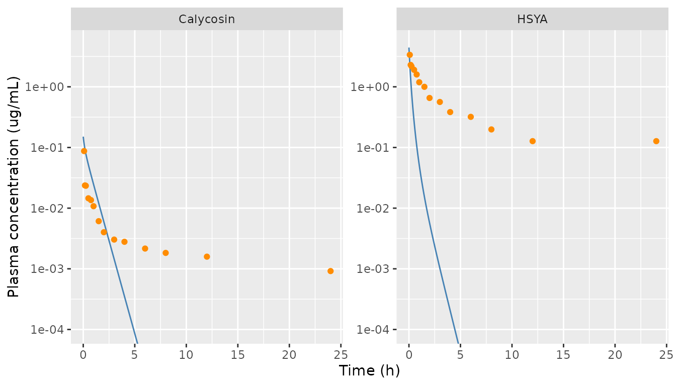
Replicates Figure 7A/E of Sun 2025: model with the printed Table 2 parameters (line) vs the mean observed concentrations (points). The published fitted curves track the points (R2 0.9830 and 0.9105); the printed parameters do not.
pk_fit <- data.frame(
  analyte = c("HSYA", "Calycosin"),
  r2_model = c(
    r2(observed$hsya, sim_obs$Cc),
    r2(observed$calycosin, sim_obs$Cc_calycosin)
  ),
  r2_paper = c(0.9830, 0.9105),
  conc_2h_model = c(sim_obs$Cc[obs_times == 2], sim_obs$Cc_calycosin[obs_times == 2]),
  conc_2h_observed = c(observed$hsya[obs_times == 2], observed$calycosin[obs_times == 2])
)
pk_fit |>
  dplyr::rename(
    "Analyte" = analyte, "R2, printed parameters" = r2_model,
    "R2, Figure 7" = r2_paper, "Model at 2 h (ug/mL)" = conc_2h_model,
    "Observed at 2 h (ug/mL)" = conc_2h_observed
  ) |>
knitr::kable(digits = 4)| Analyte | R2, printed parameters | R2, Figure 7 | Model at 2 h (ug/mL) | Observed at 2 h (ug/mL) |
|---|---|---|---|---|
| HSYA | 0.0750 | 0.9830 | 0.0057 | 0.6548 |
| Calycosin | -0.6588 | 0.9105 | 0.0059 | 0.0040 |
stopifnot(
  # The solve starts at the printed initial concentrations.
  abs(sim$Cc[1] - 4.441699) < 1e-6,
  abs(sim$Cc_calycosin[1] - 0.150838) < 1e-6,
  # The printed Table 2 parameters do not reproduce Figure 7: HSYA is
  # eliminated about 100-fold too fast by 2 h. These pin the documented
  # discrepancy; a corrected value set would trip them.
  pk_fit$r2_model[1] < 0.3,
  pk_fit$r2_model[2] < 0.3,
  sim_obs$Cc[obs_times == 2] < 0.05 * observed$hsya[obs_times == 2]
)
Figure 7 itself shows why the printed values cannot be the plotted ones: both fitted curves level off at exactly the lowest observed concentration (0.127 ug/mL for HSYA, 0.0009 ug/mL for calycosin), which an ODE with only first- and second-order elimination cannot do. The text says the concentrations were normalised before fitting and denormalised afterwards without stating how; a min-max normalisation would produce that plateau. Refitting the same ODE on the min-max scale reproduces the published R2 (about 0.99 and 0.91), but at rate constants unrelated to Table 2 (for example k~1 near 5 rather than 47), so Table 2 is not on that scale either. No reading tried by the maintainers (min-max, divide-by-maximum, -mean, -C0 or -sum normalisation, each with time in minutes, hours or days) reconciles Table 2 with Figure 7.
Mutual enhancement of elimination
The paper’s headline PK result is that each compound raises the
other’s elimination rate on average by
k~1 * mean(C2) / k1 = 30.2590% (HSYA) and
k~2 * mean(C1) / k2 = 27.7680% (calycosin) (Results, after
Eq. 20). The averaging is not defined; the table gives the value the
printed parameters imply for two readings of it.
trap <- function(x, y) sum(diff(x) * (head(y, -1) + tail(y, -1)) / 2)
kel <- 1.570177
kel_cal <- 1.413132
ks <- 47.406980
ks_cal <- 0.573247
ratio <- data.frame(
  quantity = c("HSYA: k~1 * mean(C2) / k1", "Calycosin: k~2 * mean(C1) / k2"),
  paper_pct = c(30.2590, 27.7680),
  mean_over_samples_pct = 100 * c(
    ks * mean(sim_obs$Cc_calycosin) / kel,
    ks_cal * mean(sim_obs$Cc) / kel_cal
  ),
  time_average_0_24_pct = 100 * c(
    ks * trap(sim$time, sim$Cc_calycosin) / 24 / kel,
    ks_cal * trap(sim$time, sim$Cc) / 24 / kel_cal
  )
)
ratio |>
  dplyr::rename(
    "Quantity" = quantity, "Paper (%)" = paper_pct,
    "Model, mean over sampling times (%)" = mean_over_samples_pct,
    "Model, time-average 0-24 h (%)" = time_average_0_24_pct
  ) |>
knitr::kable(digits = 2)| Quantity | Paper (%) | Model, mean over sampling times (%) | Model, time-average 0-24 h (%) |
|---|---|---|---|
| HSYA: k~1 * mean(C2) / k1 | 30.26 | 90.56 | 9.86 |
| Calycosin: k~2 * mean(C1) / k2 | 27.77 | 14.41 | 1.21 |
Neither reading reproduces both published percentages, consistent with the rate constants not being on the scale of the plotted concentrations.
Replicate Figure 8 (coupled PD)
The text states that Caspase-9 and IL-1beta were fitted after the
transform E~ = max(E) - E, but the Figure 8 fitted curves
rise and fall with the raw data, as the direct form
E = alpha E1 + beta E2 does. The model uses the direct
form.
pd_long <- sim |>
  select(time, `Caspase-9 (U/L)` = casp9, `IL-1beta (pg/mL)` = il1b, `SOD (U/mL)` = sod) |>
  pivot_longer(-time, names_to = "marker", values_to = "value")
pd_obs <- observed |>
  select(time, `Caspase-9 (U/L)` = casp9, `IL-1beta (pg/mL)` = il1b, `SOD (U/mL)` = sod) |>
  pivot_longer(-time, names_to = "marker", values_to = "value")
ggplot(pd_long, aes(time, value)) +
  geom_line(colour = "firebrick") +
  geom_point(data = pd_obs) +
  facet_wrap(~marker, scales = "free_y") +
  labs(x = "Time (h)", y = "Plasma biomarker")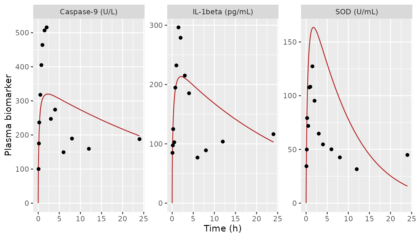
Replicates the time course behind Figure 8 of Sun 2025 (which plots response against both concentrations in 3D): model with the printed Table 4 values driven by the printed Table 2 PK (line) vs mean observed biomarker (points).
pd_fit <- data.frame(
  marker = c("Caspase-9", "IL-1beta", "SOD"),
  r2_model = c(
    r2(observed$casp9, sim_obs$casp9),
    r2(observed$il1b, sim_obs$il1b),
    r2(observed$sod, sim_obs$sod)
  ),
  r2_paper = c(0.9530, 0.9435, 0.9347),
  peak_model = c(max(sim$casp9), max(sim$il1b), max(sim$sod)),
  peak_observed = c(max(observed$casp9), max(observed$il1b), max(observed$sod))
)
pd_fit |>
  dplyr::rename(
    "Biomarker" = marker, "R2, printed parameters" = r2_model,
    "R2, Figure 8" = r2_paper, "Model peak" = peak_model,
    "Observed peak" = peak_observed
  ) |>
knitr::kable(digits = 3)| Biomarker | R2, printed parameters | R2, Figure 8 | Model peak | Observed peak |
|---|---|---|---|---|
| Caspase-9 | 0.345 | 0.953 | 320.158 | 515.712 |
| IL-1beta | 0.408 | 0.944 | 213.424 | 296.329 |
| SOD | -2.165 | 0.935 | 163.586 | 127.330 |
stopifnot(
  # Every biomarker prediction is a sum of two non-negative Hill terms bounded
  # by alpha + beta.
  all(sim$casp9 >= 0), all(sim$casp9 <= 2272.479702 + 1706.856119),
  # Driven by the printed PK, the printed PD set falls well short of the
  # published goodness of fit (R2 about 0.34, 0.41 and -2.2 against 0.93-0.95).
  all(pd_fit$r2_model < 0.6)
)
Part of this shortfall is inherited from the PK: the HSYA effect
compartments are fed by an HSYA curve that collapses within 2 h. Driving
the same Table 4 values with a PK curve that does match Figure 7 (the
min-max refit described above) raises R2 to roughly 0.88, 0.81 and 0.58,
still below Figure 8, which is consistent with Table 4 holding
single-rat rather than mean estimates (next section). Under the text’s
max(E) - E reading the same check gives R2 below -3 for all
three biomarkers.
Table 4 is single-rat estimates
The Table 4 column headed “Mean +/- Standard Deviation” equals, to all six decimals, the Caspase-9 estimates of rat 5 and the IL-1beta and SOD estimates of rat 6 in supplement Table 8. Most of the +/- values equal the across-rat SD of supplement Table 8; a few rows do not. The model carries the printed values; the true means are shown for reference.
table8 <- list(
  casp9 = rbind(
    c(0.776864, 0.054480, 3.117430, 2.468287, 5.772354, 0.000485, 5157.106153, 179.532903),
    c(0.683977, 0.000057, 2.239271, 1.732099, 2.836247, 0.131618, 2496.431586, 1848.435285),
    c(0.870005, 0.000003, 2.042384, 1.337590, 5.242619, 0.000000, 1108.685626, 277.171406),
    c(0.002985, 0.112354, 0.618366, 4.617173, 4.957217, 0.002706, 4670.019202, 2007.136639),
    c(0.785024, 0.050304, 3.108474, 1.855617, 0.539493, 0.052921, 2272.479702, 1706.856119),
    c(0.080131, 0.177727, 5.084432, 0.002150, 1.751205, 0.004458, 3290.549885, 1141.805022)
  ),
  il1b = rbind(
    c(0.435995, 10.948415, 1.189846, 4.947691, 5.278858, 0.122705, 2654.799552, 1850.439820),
    c(0.450109, 10.699612, 1.063272, 4.671586, 2.426234, 0.273618, 1943.385811, 1388.620078),
    c(0.500115, 2.239487, 0.873901, 5.230729, 5.310833, 0.574904, 1472.271501, 639.018313),
    c(0.512757, 0.009733, 3.388389, 1.828191, 0.354983, 0.468744, 2717.966258, 1584.625300),
    c(0.556277, 0.002545, 1.436247, 4.891564, 0.222948, 0.938191, 2314.627344, 671.014691),
    c(0.481205, 0.075605, 5.309134, 1.297095, 0.512179, 0.139198, 2141.182784, 1382.785005)
  ),
  sod = rbind(
    c(0.785710, 0.001220, 0.957266, 4.467441, 5.909932, 0.344594, 566.700991, 180.253022),
    c(1.427625, 0.117812, 5.854821, 5.403171, 2.088358, 0.005848, 1273.297490, 954.626422),
    c(0.959824, 0.135082, 2.560980, 2.841333, 0.313225, 0.454334, 759.180176, 292.724042),
    c(0.600947, 0.115378, 4.887875, 2.686980, 2.399895, 0.003224, 515.399488, 395.412738),
    c(0.959983, 0.121288, 2.660851, 2.765058, 0.414881, 0.527100, 733.822828, 551.176094),
    c(0.872465, 0.141701, 5.241084, 1.846627, 0.861183, 0.026937, 866.979600, 600.197532)
  )
)
table4_sd <- list(
  casp9 = c(0.386098, 0.038869, 1.483545, 1.522608, 0.725352, 0.042906, 1531.099793, 803.111331),
  il1b = c(0.043809, 0.058495, 1.773854, 1.158816, 0.417957, 0.110984, 466.228288, 493.523387),
  sod = c(0.276299, 0.052074, 1.914617, 1.323894, 0.202854, 0.012725, 271.578691, 273.99794)
)
param_rows <- c("ke1", "ke2", "gamma1", "EC50_1", "gamma2", "EC50_2", "alpha", "beta")
ini_names <- function(m) {
  c(
    paste0("lke0_", m), paste0("lke0_", m, "_calycosin"),
    paste0("lhill_", m), paste0("lec50_", m),
    paste0("lhill_", m, "_calycosin"), paste0("lec50_", m, "_calycosin"),
    paste0("lemax_", m), paste0("lemax_", m, "_calycosin")
  )
}
theta <- setNames(mod_rx$theta, names(mod_rx$theta))
table4_check <- bind_rows(lapply(names(table8), function(m) {
  data.frame(
    marker = m,
    parameter = param_rows,
    model_value = exp(theta[ini_names(m)]),
    true_mean = colMeans(table8[[m]]),
    printed_sd = table4_sd[[m]],
    true_sd = apply(table8[[m]], 2, sd)
  )
}))
table4_check |>
  dplyr::rename(
    "Biomarker" = marker, "Parameter" = parameter,
    "Model (= Table 4 'Mean')" = model_value,
    "Mean of supplement Table 8" = true_mean,
    "Table 4 +/- SD" = printed_sd,
    "SD of supplement Table 8" = true_sd
  ) |>
knitr::kable(digits = 4, row.names = FALSE)| Biomarker | Parameter | Model (= Table 4 ‘Mean’) | Mean of supplement Table 8 | Table 4 +/- SD | SD of supplement Table 8 |
|---|---|---|---|---|---|
| casp9 | ke1 | 0.7850 | 0.5332 | 0.3861 | 0.3861 |
| casp9 | ke2 | 0.0503 | 0.0658 | 0.0389 | 0.0689 |
| casp9 | gamma1 | 3.1085 | 2.7017 | 1.4835 | 1.4835 |
| casp9 | EC50_1 | 1.8556 | 2.0022 | 1.5226 | 1.5226 |
| casp9 | gamma2 | 0.5395 | 3.5165 | 0.7254 | 2.1254 |
| casp9 | EC50_2 | 0.0529 | 0.0320 | 0.0429 | 0.0529 |
| casp9 | alpha | 2272.4797 | 3165.8787 | 1531.0998 | 1531.0998 |
| casp9 | beta | 1706.8561 | 1193.4896 | 803.1113 | 803.1113 |
| il1b | ke1 | 0.4812 | 0.4894 | 0.0438 | 0.0438 |
| il1b | ke2 | 0.0756 | 3.9959 | 0.0585 | 5.3585 |
| il1b | gamma1 | 5.3091 | 2.2101 | 1.7739 | 1.7739 |
| il1b | EC50_1 | 1.2971 | 3.8111 | 1.1588 | 1.7588 |
| il1b | gamma2 | 0.5122 | 2.3510 | 0.4180 | 2.4180 |
| il1b | EC50_2 | 0.1392 | 0.4196 | 0.1110 | 0.3110 |
| il1b | alpha | 2141.1828 | 2207.3722 | 466.2283 | 466.2283 |
| il1b | beta | 1382.7850 | 1252.7505 | 493.5234 | 493.5234 |
| sod | ke1 | 0.8725 | 0.9344 | 0.2763 | 0.2763 |
| sod | ke2 | 0.1417 | 0.1054 | 0.0521 | 0.0521 |
| sod | gamma1 | 5.2411 | 3.6938 | 1.9146 | 1.9146 |
| sod | EC50_1 | 1.8466 | 3.3351 | 1.3239 | 1.3239 |
| sod | gamma2 | 0.8612 | 1.9979 | 0.2029 | 2.1029 |
| sod | EC50_2 | 0.0269 | 0.2270 | 0.0127 | 0.2427 |
| sod | alpha | 866.9796 | 785.8968 | 271.5787 | 271.5787 |
| sod | beta | 600.1975 | 495.7316 | 273.9979 | 273.9979 |
single_rat <- c(casp9 = 5L, il1b = 6L, sod = 6L)
stopifnot(
  all(vapply(names(table8), function(m) {
    max(abs(exp(theta[ini_names(m)]) / table8[[m]][single_rat[[m]], ] - 1)) < 1e-6
  }, logical(1))),
  # Table 4 rows 9-10 (eta1) follow from alpha / (alpha + beta) as Eq. 6 states.
  abs(2272.479702 / (2272.479702 + 1706.856119) - 0.57107) < 1e-5,
  abs(2141.182784 / (2141.182784 + 1382.785005) - 0.607606) < 1e-6,
  abs(866.9796 / (866.9796 + 600.197532) - 0.590917) < 1e-6
)
PKNCA validation against Table 3
Table 3 reports PK indices that the paper says were computed from the fitted central-compartment concentrations. NCA of the packaged model (one typical rat, dense grid from time 0) is compared with them below.
nca_conc <- bind_rows(
  sim |> transmute(id = 1L, analyte = "HSYA", time, Cc),
  sim |> transmute(id = 1L, analyte = "Calycosin", time, Cc = Cc_calycosin)
) |>
  dplyr::filter(!is.na(Cc))
conc_obj <- PKNCA::PKNCAconc(nca_conc, Cc ~ time | analyte + id)
intervals <- data.frame(
  start = 0, end = 24,
  auclast = TRUE, aucinf.obs = TRUE, half.life = TRUE
)
nca_res <- PKNCA::pk.nca(PKNCA::PKNCAdata(conc_obj, intervals = intervals))
#> No dose information provided, calculations requiring dose will return NA.

published_nca <- data.frame(
  analyte = c("HSYA", "Calycosin"),
  auclast = c(3.722933, 0.081207),
  aucinf.obs = c(3.846167, 0.081864),
  half.life = c(0.227083, 0.255)
)
nca_cmp <- nlmixr2lib::ncaComparisonTable(
  simulated = nca_res,
  reference = published_nca,
  by = "analyte",
  units = c(auclast = "ug*h/mL", aucinf.obs = "ug*h/mL", half.life = "h"),
  tolerance_pct = 20
)
knitr::kable(
  nca_cmp,
  caption = "Packaged model vs Sun 2025 Table 3. * differs from the published value by >20%."
)| NCA parameter | analyte | Reference | Simulated | % diff |
|---|---|---|---|---|
| AUC0-∞ (obs) (ug*h/mL) | HSYA | 3.85 | 0.714 | -81.4%* |
| AUC0-∞ (obs) (ug*h/mL) | Calycosin | 0.0819 | 0.0783 | -4.3% |
| AUClast (ug*h/mL) | HSYA | 3.72 | 0.714 | -80.8%* |
| AUClast (ug*h/mL) | Calycosin | 0.0812 | 0.0783 | -3.5% |
| t½ (h) | HSYA | 0.227 | 0.439 | +93.5%* |
| t½ (h) | Calycosin | 0.255 | 0.49 | +92.2%* |
Only the calycosin AUCs agree (within 5%); the HSYA AUCs and both
half-lives differ by more than 80%. Table 3 also gives MRT0-t of 8.22 h
(HSYA) and 9.67 h (calycosin), whereas the model concentrations fall
below 1% of their initial value within about 3 h. The Table 3 values are
not derivable from the printed model: an HSYA MRT of 8.97 h is
incompatible with a terminal half-life of 0.227 h in a one-compartment
system, and the HSYA AUC0-inf of 3.85 ug*h/mL exceeds
C10 / k1 = 2.83 ug*h/mL, the AUC the printed
HSYA disposition would give even with no calycosin present. They do not
match an NCA of the observed mean data either (trapezoidal HSYA AUC from
0.083 to 24 h is about 7.2 ug*h/mL).
nca_tbl <- as.data.frame(nca_res)
model_auc_hsya <- nca_tbl$PPORRES[nca_tbl$analyte == "HSYA" & nca_tbl$PPTESTCD == "auclast"]
stopifnot(
  # Structural check: the printed parameters give an HSYA AUC0-24 near
  # 0.71 ug*h/mL, below the no-interaction ceiling C10 / k1.
  abs(model_auc_hsya - 0.714) < 0.01,
  model_auc_hsya < 4.441699 / 1.570177
)
Assumptions and deviations
- Parameters carried verbatim (Errata). The printed Table 2 and Table 4 values are used unchanged, by the maintainers’ decision, even though they do not reproduce the paper’s figures. Nothing was refitted or tuned. The alternative was to omit the paper; carrying it with the discrepancies quantified keeps the structure (mutual concentration-dependent elimination with dual effect compartments) available and auditable.
- Table 2 does not reproduce Figure 7 (Errata). With the printed values the model predicts HSYA falling to 0.006 ug/mL at 2 h against 0.65 observed (R2 about 0.08 for HSYA and negative for calycosin, against 0.983 and 0.911 in Figure 7). The unspecified normalisation is the likely cause. Table 2 does equal the arithmetic mean of the per-rat estimates in supplement Table 6, so the transcription is faithful.
- Table 4 ‘Mean’ column is single-rat values (Errata). It equals rat 5 (Caspase-9) and rat 6 (IL-1beta, SOD) of supplement Table 8. The printed values are used; the true means are tabulated above for anyone who prefers them.
-
PD observation form. The direct form
E = alpha E1 + beta E2is used for all three biomarkers, following Figure 8 and Eq. 5/7; the text’smax(E) - Etransform for Caspase-9 and IL-1beta contradicts Figure 8 and would need the unreportedmax(E). -
Sign of the coupling constants. The supplementary
stability analysis requires
k~1, k~2 < 0, but Table 2 prints them positive and the text concludes that the compounds enhance each other’s metabolism. The printed positive values are used;ksandks_calycosinare kept on the linear scale so a user can test the other sign. -
No dose input. The model has concentration states
initialised at
C10andC20; it describes only the studied 2 + 1 mg/kg co-injection. Scaling to another dose would assume dose-proportional initial concentrations, which the paper does not test. - No variability. The paper fitted the six-rat mean (and each rat separately) with a per-time-point likelihood; no IIV or residual error was estimated, so all residual SDs are fixed at 0. The across-rat SDs of Tables 2 and 4 are not converted into IIV.
- Table 3 PK indices match neither the model (apart from the calycosin AUCs) nor the observed data and are not used.