Ritlecitinib safety exposure-response: QTc, lymphocytes, infections, herpes zoster and rash (Huh 2025)
Source:vignettes/articles/Huh_2025_ritlecitinib_safety.Rmd
Huh_2025_ritlecitinib_safety.RmdModel and source
- Citation: Huh Y, Qiu R, Prybylski J, Wojciechowski J, Wang Y, Purohit VS. Comprehensive Safety Exposure-Response Analysis to Support Ritlecitinib Dose Selection. CPT Pharmacometrics Syst Pharmacol. 2025;14(6):1108-1118. doi:10.1002/psp4.70030. PK layer from Wojciechowski J, Purohit VS, Huh Y, Banfield C, Nicholas T. Evolution of Ritlecitinib Population Pharmacokinetic Models During Clinical Drug Development. Clin Pharmacokinet. 2023;62(12):1765-1779. doi:10.1007/s40262-023-01318-3 (final-model column of Table 2; see modellib(‘Wojciechowski_2023_ritlecitinib_final’)).
- Article: https://doi.org/10.1002/psp4.70030
Huh et al. (2025) characterised the safety of ritlecitinib, a JAK3/TEC-family kinase inhibitor approved for alopecia areata in adults and adolescents, with five separately fitted exposure-response models. The package carries one file for each:
| Model file | Endpoint | Output | Structure | Source |
|---|---|---|---|---|
Huh_2025_ritlecitinib_QTcF |
Change from baseline in QTcF (ms) | QTcF |
Garnett white-paper linear mixed-effects C-QTc model | Equation 1, Table 2 |
Huh_2025_ritlecitinib_lymphocytes |
Absolute lymphocyte count (10^9/L) | circ |
Friberg proliferation / 3-transit / circulation model with an Emax drug effect, driven by the embedded Wojciechowski 2023 PK model | Equation 2, Table 2, Supplement 2 |
Huh_2025_ritlecitinib_infections |
First infection adverse event | infection_count |
Poisson regression with log(time) offset on sqrt(time-weighted Cave) | Equation 3, Table 2 |
Huh_2025_ritlecitinib_herpes_zoster |
First herpes zoster event | herpes_zoster_count |
as above | Equation 3, Table 2 |
Huh_2025_ritlecitinib_rash |
First rash adverse event | rash_count |
as above | Equation 3, Table 2 |
The longitudinal efficacy (SALT score) model the paper combines with
these in its benefit:risk figure is Huh_2024_ritlecitinib,
and the population PK model whose individual estimates drove every
exposure metric is
Wojciechowski_2023_ritlecitinib_final.
Population
- C-QTc: 946 post-baseline ECG observations from 79 healthy volunteers in the single-ascending-dose period (5-800 mg or placebo) of the first-in-human study B7981001 (Results; Table 1).
- Lymphocytes: 1958 subjects, 80 healthy volunteers from B7981001 and 1878 adolescent and adult alopecia areata patients from the phase 2a (B7931005), phase 2b/3 (B7981015) and phase 3 long-term (B7981032) studies, aged 12-72 years (Results; Tables 1 and 3).
- Adverse events: 1744 subjects (121 healthy volunteers, 1259 alopecia areata and 364 vitiligo patients) from five phase 1 studies, the three alopecia areata studies and the phase 2b vitiligo study B7981019; 241, 22 and 434 subjects had at least one infection, herpes zoster or rash event, respectively (Results; Table 1; preferred terms in Table S1).
Sex, weight and race distributions of the analysis datasets are not
reported. The population element of each model holds these
facts, e.g.
readModelDb("Huh_2025_ritlecitinib_rash")()$population.
Source trace
Every ini() value carries an in-file comment naming its
source. The tables below collect them.
C-QTc model (Table 2, ‘Concentration-QTc model’)
| Parameter | Value | Source |
|---|---|---|
e0 (intercept, placebo, 0.5 h) |
-2.76 ms | Table 2 ‘Intercept’ |
e_ntime1_e0 … e_ntime24_e0
|
0.702, 1.91, 1.16, -2.73, 1.09, 1.96, 2.25 ms | Table 2 ‘Time effect’ rows (1, 2, 4, 8, 12, 16, 24 h) |
e_on_treatment_e0 |
-0.354 ms | Table 2 ‘Treatment effect’ |
e_qtc_bl_e0 |
-0.208 | Table 2 ‘Baseline effect’ |
slope |
0.000213 ms per ng/mL | Table 2 ‘Slope’; Results ‘0.213 ms … per 1000 ng/mL’ |
etae0, etaslope
|
SD 4.37 ms and 3.75e-7 ms per ng/mL, correlation 5.84e-5 | Table 2 omega rows (read as nlme SDs and a correlation; see Assumptions) |
addSd |
5.05 ms | Table 2 ‘Residual Variability’ |
| Structure | linear in C, TRT, centered baseline and nominal-time factor | Equation 1; Supplement 2 nlme call |
Lymphocyte PK/PD model (Table 2, ‘Lymphocyte PK/PD model’; Supplement 2)
| Parameter | Value | Source |
|---|---|---|
lcirc0 |
1.65 x 10^9/L | Table 2 ‘Circ 0’ |
e_age_circ0 |
-0.153 (power of AGE/45) | Table 2; Results equation circ0 = pop x (Age/45)^-0.153 |
e_sexf_circ0 |
0.0609 | Table 2 ‘Effect of Female on Circ 0’; Results ‘6% higher’ |
lmtt |
3.12 days | Table 2 ‘MTT’ |
lgamma |
0.0154 | Table 2 ‘gamma’ |
lemax |
1 (fixed) | Table 2 ‘E max 1 fix’ |
e_circ0_emax |
-1.6 | Table 2; Results Emax = pop Emax x (circ0/pop circ0)^-1.6 |
lec50 |
25,800 ng/mL | Table 2 ‘EC 50’ |
etalcirc0 |
0.0493 | Table 2 ‘omega^2 CIRC0’ |
propSd |
0.187 | Table 2 ‘Residual Error’; Supplement 2 $ERROR (proportional, $SIGMA 1 FIX) |
| ntrans = 3, kprol = ktr = kcirc = 4/MTT | Equation 2 and text | |
| Effect cap EDRUG <= 1 | Supplement 2 $DES | |
PK layer (lcl … etalvc) |
Wojciechowski 2023 final model, all fixed | Methods (‘EBE of individual PK parameters from the population PK
model [11]’); Wojciechowski_2023_ritlecitinib_final
|
Adverse-event Poisson models (Table 2)
| Model | Parameter | Value | Source |
|---|---|---|---|
| Infections | lbase |
-9.00 | Table 2 ‘Intercept (theta 0)’ |
| Infections | e_region_asia_lbase |
-1.31 | Table 2 ‘Effect of Asia (geographical location)’ |
| Infections | e_sexf_lbase |
0.748 | Table 2 ‘Effect of female sex’ |
| Infections | slope |
0.0989 per sqrt(ng/mL) | Table 2 ‘Slope (theta Cave)’ |
| Herpes zoster | lbase |
-11.3 | Table 2 |
| Herpes zoster | e_age_lbase |
0.0396 per year | Table 2 ‘Effect of age (referenced to 34 years)’ |
| Herpes zoster | slope |
0.0873 per sqrt(ng/mL) | Table 2 |
| Rash | lbase |
-6.02 | Table 2 |
| Rash | e_alopecia_areata_lbase |
-2.86 | Table 2 ‘Effect of AA patients’ |
| Rash | e_vitiligo_lbase |
-2.73 | Table 2 ‘Effect of Vitiligo patients’ |
| Rash | e_region_asia_lbase |
0.632 | Table 2 |
| Rash | e_age_lbase |
-0.0185 per year | Table 2 |
| Rash | e_sexf_lbase |
0.521 | Table 2 |
| Rash | slope |
0.142 per sqrt(ng/mL) | Table 2 |
| All | log(lambda) = theta0 + log(t) + slope x sqrt(Cave) + covariates | Equation 3; square root selected by AIC (Supplement 2) |
Concentration-QTc model
The model predicts the change from baseline in QTcF. Its placebo-corrected, time-matched effect is the difference between an active and a placebo record at the same nominal time, which cancels the intercept, the time effects and the baseline term: DeltaDeltaQTcF = theta2 + theta1 x C.
mod_qtc <- readModelDb("Huh_2025_ritlecitinib_QTcF")

conc_grid <- c(0, 100, 500, 1000, 2000, 3000, 4000, 5000)
qtc_ev <- bind_rows(
  data.frame(CP_RITLECITINIB_NGML = conc_grid, ON_TREATMENT = 1),
  data.frame(CP_RITLECITINIB_NGML = 0, ON_TREATMENT = 0)
) |>
  mutate(
    id = 1L,
    time = seq_len(n()),
    evid = 0L,
    amt = 0,
    NTIME = 2,
    QTC_BL = 400
  )

qtc_sim <- rxSolve(rxode2::zeroRe(mod_qtc), qtc_ev, returnType = "data.frame")
#> ℹ omega/sigma items treated as zero: 'etae0', 'etaslope'

placebo_dqtc <- qtc_sim$QTcF[qtc_ev$ON_TREATMENT == 0]
ddqtc <- qtc_sim |>
  filter(ON_TREATMENT == 1) |>
  transmute(
    conc = CP_RITLECITINIB_NGML,
    ddqtc_model = QTcF - placebo_dqtc,
    ddqtc_closed = -0.354 + 0.000213 * conc
  )

# A typical solve against its own closed form: pure arithmetic, so the bound
# is tight.
stopifnot(max(abs(ddqtc$ddqtc_model - ddqtc$ddqtc_closed)) < 1e-8)
# Results: 'only a 0.213 ms increase in QTcF per 1000 ng/mL'.
stopifnot(abs(diff(ddqtc$ddqtc_model[ddqtc$conc %in% c(0, 1000)]) - 0.213) < 1e-8)

ddqtc |>
  dplyr::rename(
    "Ritlecitinib (ng/mL)" = conc,
    "DeltaDeltaQTcF, model (ms)" = ddqtc_model,
    "theta2 + theta1 x C (ms)" = ddqtc_closed
  ) |>
knitr::kable(digits = 3)| Ritlecitinib (ng/mL) | DeltaDeltaQTcF, model (ms) | theta2 + theta1 x C (ms) |
|---|---|---|
| 0 | -0.354 | -0.354 |
| 100 | -0.333 | -0.333 |
| 500 | -0.248 | -0.248 |
| 1000 | -0.141 | -0.141 |
| 2000 | 0.072 | 0.072 |
| 3000 | 0.285 | 0.285 |
| 4000 | 0.498 | 0.498 |
| 5000 | 0.711 | 0.711 |
The point estimate stays below 1 ms across the whole concentration range of the single-ascending-dose study, consistent with the paper’s conclusion of no ritlecitinib-induced QTc prolongation. The paper’s 4.13 ms is the upper bound of the 90% confidence interval at the 800 mg Cmax, which needs the parameter covariance matrix and cannot be reproduced from the published estimates.
qtc_time_ev <- tidyr::expand_grid(
  NTIME = c(0.5, 1, 2, 4, 8, 12, 16, 24),
  ON_TREATMENT = c(0, 1)
) |>
  mutate(
    CP_RITLECITINIB_NGML = 1000 * ON_TREATMENT,
    QTC_BL = 400,
    id = 1L,
    time = seq_len(n()),
    evid = 0L,
    amt = 0
  )
qtc_time <- rxSolve(rxode2::zeroRe(mod_qtc), qtc_time_ev, returnType = "data.frame")
#> ℹ omega/sigma items treated as zero: 'etae0', 'etaslope'
ggplot(
  qtc_time,
  aes(NTIME, QTcF, colour = factor(ON_TREATMENT, labels = c("Placebo", "Ritlecitinib 1000 ng/mL")))
) +
  geom_point() +
  geom_line() +
  labs(x = "Nominal time after dose (h)", y = "Typical DeltaQTcF (ms)", colour = NULL) +
  theme_bw()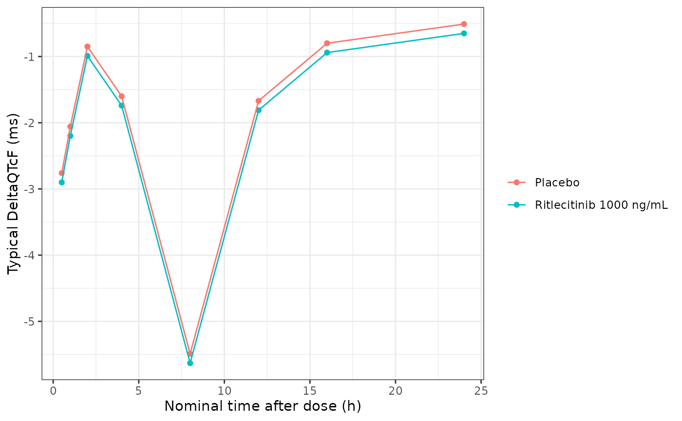
Typical change from baseline in QTcF by nominal time for placebo and for a 1000 ng/mL ritlecitinib concentration (QTC_BL = 400 ms). The time pattern is the theta_k diurnal shifts of Table 2.
Lymphocyte PK/PD model
Virtual cohort
The analysis dataset demographics are not reported, so the cohort follows the alopecia areata population of the Wojciechowski 2023 final PK model (median weight 68.5 kg, range 29.6-131 kg; 60.6% female) with an age mix spanning the paper’s three age subgroups (12-17, 18-50 and 51-72 years). Each arm has 150 subjects.
mod_lym <- readModelDb("Huh_2025_ritlecitinib_lymphocytes")

make_cohort <- function(n, arm, id_offset) {
  u <- runif(n)
  data.frame(
    id = id_offset + seq_len(n),
    arm = arm,
    AGE = ifelse(
      u < 0.15,
      runif(n, 12, 17.99),
      ifelse(u < 0.80, runif(n, 18, 50.99), runif(n, 51, 72))
    ),
    WT = pmin(pmax(exp(rnorm(n, log(68.5), 0.22)), 29.6), 131),
    SEXF = rbinom(n, 1, 0.606),
    DIS_ALOPECIA_AREATA = 1
  )
}

# Regimens of the phase 2b/3 study (Figure 2) plus 100 and 200 mg QD (Figure 4).
regimens <- data.frame(
  arm = c("Placebo", "10 mg", "30 mg", "50 mg", "100 mg", "200 mg",
          "200 mg x4w, 30 mg", "200 mg x4w, 50 mg"),
  load = c(0, 0, 0, 0, 0, 0, 200, 200),
  maint = c(0, 10, 30, 50, 100, 200, 30, 50)
)
n_arm <- 150
set.seed(20250512)
cohort <- bind_rows(lapply(seq_len(nrow(regimens)), function(i) {
  make_cohort(n_arm, regimens$arm[i], (i - 1) * n_arm)
})) |>
  left_join(regimens, by = "arm")
Steady-state exposure (PKNCA)
The adverse-event models need the time-weighted average concentration, so the embedded PK layer is checked first against the paper’s geometric mean steady-state Cave of 27 ng/mL at 30 mg QD and 257 ng/mL at 200 mg QD (Results, infections paragraph). Cave is taken over day 14 (steady state; half-life 1.3-2.3 h).
pk_cohort <- cohort |> filter(load == 0, maint %in% c(30, 50, 100, 200))
pk_obs_t <- c(0, seq(312, 336, by = 0.25))
pk_ev <- bind_rows(lapply(seq_len(nrow(pk_cohort)), function(i) {
  rbind(
    data.frame(id = pk_cohort$id[i], time = 0, amt = pk_cohort$maint[i], ii = 24,
               addl = 13, evid = 1, cmt = "depot"),
    data.frame(id = pk_cohort$id[i], time = pk_obs_t, amt = 0, ii = 0, addl = 0,
               evid = 0, cmt = "central")
  )
})) |>
  left_join(pk_cohort |> select(id, AGE, WT, SEXF, DIS_ALOPECIA_AREATA), by = "id") |>
  arrange(id, time, desc(evid))

rxode2::rxSetSeed(20250512)
pk_sim <- rxSolve(mod_lym, pk_ev, maxsteps = 1e6, returnType = "data.frame") |>
  left_join(pk_cohort |> select(id, arm), by = "id")
#> ℹ parameter labels from comments will be replaced by 'label()'
#> Warning: some etas defaulted to non-mu referenced, possible parsing error: etalcl, etalvc
#> as a work-around try putting the mu-referenced expression on a simple line

pk_conc <- pk_sim |>
  filter(!is.na(Cc)) |>
  select(id, arm, time, Cc)
pk_dose <- pk_ev |>
  filter(evid == 1) |>
  left_join(pk_cohort |> select(id, arm), by = "id") |>
  select(id, arm, time, amt)

nca_data <- PKNCAdata(
  PKNCAconc(pk_conc, Cc ~ time | arm + id),
  PKNCAdose(pk_dose, amt ~ time | arm + id),
  intervals = data.frame(start = 312, end = 336, cav = TRUE, cmax = TRUE)
)
nca_res <- pk.nca(nca_data)

# The paper reports geometric means, so aggregate the same way before the
# comparison (ncaComparisonTable() would otherwise take the median).
cav_gm <- as.data.frame(nca_res) |>
  filter(PPTESTCD == "cav") |>
  group_by(arm, PPTESTCD) |>
  summarise(PPORRES = exp(mean(log(PPORRES))), .groups = "drop")

cav_ref <- data.frame(arm = c("30 mg", "200 mg"), cav = c(27, 257))
cmp_cav <- nlmixr2lib::ncaComparisonTable(
  cav_gm |> filter(arm %in% cav_ref$arm),
  cav_ref,
  by = "arm",
  units = c(cav = "ng/mL")
)
knitr::kable(cmp_cav, caption = "Geometric mean steady-state Cave: simulated versus Huh 2025 Results.")| NCA parameter | arm | Reference | Simulated | % diff |
|---|---|---|---|---|
| Cavg (ng/mL) | 30 mg | 27 | 25.3 | -6.1% |
| Cavg (ng/mL) | 200 mg | 257 | 247 | -3.7% |
# Centre statistic of 150 subjects per arm; the paper's 10,000-patient
# geometric means are reproduced within a few percent.
cav_chk <- cav_gm |> inner_join(cav_ref, by = "arm")
stopifnot(all(abs(cav_chk$PPORRES / cav_chk$cav - 1) < 0.15))
Geometric mean Cave at 50 mg QD is 50.1 ng/mL in this cohort.
Typical time course and the steady-state reduction
With kprol = ktr and E far below 1, the steady state of the Friberg chain satisfies (1 - E)(circ0/circ)^gamma = 1, so with an oscillating concentration the steady-state count is circ0 x exp(mean(log(1 - E(t))) / gamma). A typical 70 kg, 45-year-old male patient (circ0 = 1.65 x 10^9/L, Emax = 1) is solved for two years at 50 mg QD and compared against that expression.
typ_ev <- rbind(
  data.frame(id = 1, time = 0, amt = 50, ii = 24, addl = 729, evid = 1, cmt = "depot"),
  data.frame(id = 1, time = seq(0, 730 * 24, by = 24), amt = 0, ii = 0, addl = 0,
             evid = 0, cmt = "circ"),
  data.frame(id = 1, time = seq(729 * 24, 730 * 24, by = 0.1), amt = 0, ii = 0,
             addl = 0, evid = 0, cmt = "circ")
) |>
  mutate(WT = 70, AGE = 45, SEXF = 0, DIS_ALOPECIA_AREATA = 1) |>
  arrange(time, desc(evid)) |>
  distinct(time, evid, .keep_all = TRUE)
typ <- rxSolve(rxode2::zeroRe(mod_lym), typ_ev, maxsteps = 1e6, returnType = "data.frame")
#> ℹ parameter labels from comments will be replaced by 'label()'
#> Warning: some etas defaulted to non-mu referenced, possible parsing error: etalcl, etalvc
#> as a work-around try putting the mu-referenced expression on a simple line
#> Warning: some etas defaulted to non-mu referenced, possible parsing error: etalcl, etalvc
#> as a work-around try putting the mu-referenced expression on a simple line
#> ℹ omega/sigma items treated as zero: 'etalcl', 'etalvc', 'etalcirc0'

last_day <- typ |> filter(time >= 729 * 24)
ss_closed <- 1.65 * exp(mean(log(1 - last_day$edrug)) / 0.0154)
ss_model <- mean(last_day$circ)
c(model = ss_model, closed_form = ss_closed)
#>       model closed_form
#>    1.449781    1.450441
# The chain relaxes on a ~1/(ktr * gamma) = 50-day time scale, so two years is
# at steady state; the residual difference is the averaging grid.
stopifnot(abs(ss_model / ss_closed - 1) < 0.01)
ggplot(typ |> filter(time %% 24 == 0, time <= 365 * 24), aes(time / 24 / 7, circ)) +
  geom_line() +
  labs(x = "Time after first dose (weeks)", y = "Lymphocytes (10^9/L)") +
  theme_bw()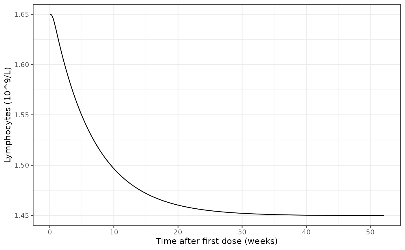
Typical lymphocyte count of a 45-year-old male patient (baseline 1.65 x 10^9/L) during 50 mg QD dosing.
Visual predictive check by regimen (Figure 2)
obs_t <- seq(0, 52 * 7 * 24, by = 24)
make_events <- function(row) {
  doses <- if (row$maint == 0) {
    NULL
  } else if (row$load > 0) {
    rbind(
      data.frame(id = row$id, time = 0, amt = row$load, ii = 24, addl = 27,
                 evid = 1, cmt = "depot"),
      data.frame(id = row$id, time = 28 * 24, amt = row$maint, ii = 24,
                 addl = 52 * 7 - 29, evid = 1, cmt = "depot")
    )
  } else {
    data.frame(id = row$id, time = 0, amt = row$maint, ii = 24, addl = 52 * 7 - 1,
               evid = 1, cmt = "depot")
  }
  rbind(
    doses,
    data.frame(id = row$id, time = obs_t, amt = 0, ii = 0, addl = 0, evid = 0,
               cmt = "circ")
  )
}
lym_ev <- bind_rows(lapply(split(cohort, cohort$id), make_events)) |>
  left_join(cohort |> select(id, AGE, WT, SEXF, DIS_ALOPECIA_AREATA), by = "id") |>
  arrange(id, time, desc(evid))

rxode2::rxSetSeed(20250513)
lym_sim <- rxSolve(mod_lym, lym_ev, maxsteps = 1e6, returnType = "data.frame") |>
  left_join(cohort |> select(id, arm), by = "id")
fig2_arms <- c("200 mg x4w, 50 mg", "200 mg x4w, 30 mg", "50 mg", "30 mg", "10 mg", "Placebo")
vpc <- lym_sim |>
  filter(arm %in% fig2_arms, time %% (7 * 24) == 0) |>
  mutate(week = time / (7 * 24), arm = factor(arm, levels = fig2_arms)) |>
  group_by(arm, week) |>
  summarise(
    p05 = quantile(sim, 0.05),
    p50 = median(sim),
    p95 = quantile(sim, 0.95),
    .groups = "drop"
  )
ggplot(vpc, aes(week)) +
  geom_line(aes(y = p50), colour = "red") +
  geom_line(aes(y = p05), colour = "steelblue") +
  geom_line(aes(y = p95), colour = "steelblue") +
  facet_wrap(~arm, nrow = 1) +
  coord_cartesian(ylim = c(0, 4)) +
  labs(x = "Time after first dose (weeks)", y = expression("Lymphocyte count (" * 10^9 * "/L)")) +
  theme_bw()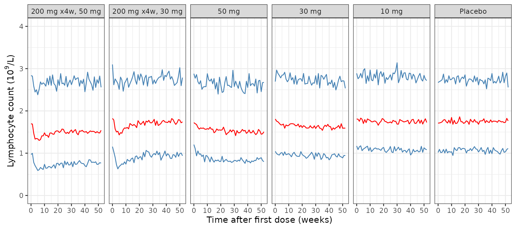
Replicates Figure 2 of Huh 2025: simulated median and 5th/95th percentiles of the lymphocyte count (with residual error) by phase 2b/3 regimen.
late_median <- vpc |>
  filter(week >= 24) |>
  group_by(arm) |>
  summarise(median_wk24_52 = median(p50), p05 = median(p05), p95 = median(p95))
knitr::kable(late_median, digits = 2,
caption = "Simulated percentiles averaged over weeks 24-52.")| arm | median_wk24_52 | p05 | p95 |
|---|---|---|---|
| 200 mg x4w, 50 mg | 1.51 | 0.77 | 2.69 |
| 200 mg x4w, 30 mg | 1.74 | 0.96 | 2.79 |
| 50 mg | 1.50 | 0.82 | 2.61 |
| 30 mg | 1.60 | 0.94 | 2.69 |
| 10 mg | 1.75 | 1.07 | 2.82 |
| Placebo | 1.75 | 1.07 | 2.72 |
Figure 2 of the paper shows medians of about 1.5 x 10^9/L for the 50 mg arms (with and without loading), about 1.6 for 30 mg, about 1.75 for 10 mg and about 1.9 for placebo, with 5th and 95th percentiles near 0.8 and 2.6-2.8. The simulated percentiles fall in the same places.
med_50 <- late_median$median_wk24_52[late_median$arm == "50 mg"]
med_pbo <- late_median$median_wk24_52[late_median$arm == "Placebo"]
# Centre of a 150-subject arm; read off Figure 2 at ~1.5 (50 mg) and ~1.9
# (placebo), a separation well beyond the cohort noise.
stopifnot(med_50 > 1.3, med_50 < 1.75, med_pbo > med_50 + 0.1)
Covariate subgroups and lymphopenia (Table 3, Figure 4)
per_subj <- lym_sim |>
  group_by(id, arm) |>
  summarise(
    baseline = circ[time == 0],
    nadir = min(circ),
    AGE = AGE[1],
    .groups = "drop"
  ) |>
  mutate(
    pcfb = 100 * (nadir / baseline - 1),
    grade34 = nadir < 0.5,
    bl_group = cut(baseline, c(0, 1.6, 2.0, Inf), right = FALSE,
                   labels = c("< 1.6", "1.6-2.0", "> 2.0")),
    age_group = cut(AGE, c(12, 18, 51, 73), right = FALSE,
                    labels = c("12-17 years", "18-50 years", "51-72 years"))
  )

tab3_bl <- per_subj |>
  filter(arm == "50 mg") |>
  group_by(bl_group) |>
  summarise(n = n(), sim_pcfb = median(pcfb), sim_grade34 = 100 * mean(grade34)) |>
  mutate(
    paper_pcfb = c("-20.5 (-24.4, -15.3)", "-15.5 (-20.5, -7.1)", "-11.4 (-17.8, 0.0)"),
    paper_grade34 = c("0.0 (0.0, 1.7)", "0.0 (0.0, 0.0)", "0.0 (0.0, 0.0)")
  )
tab3_bl |>
  dplyr::rename(
    "Baseline (10^9/L)" = bl_group,
    "Simulated median change at nadir (%)" = sim_pcfb,
    "Simulated grade 3/4 (%)" = sim_grade34,
    "Huh 2025 change from baseline (%)" = paper_pcfb,
    "Huh 2025 grade 3/4 (%)" = paper_grade34
  ) |>
knitr::kable(digits = 1, caption = "Replicates the lymphopenia baseline rows of Table 3 (50 mg QD).")| Baseline (10^9/L) | n | Simulated median change at nadir (%) | Simulated grade 3/4 (%) | Huh 2025 change from baseline (%) | Huh 2025 grade 3/4 (%) |
|---|---|---|---|---|---|
| < 1.6 | 49 | -16.1 | 0 | -20.5 (-24.4, -15.3) | 0.0 (0.0, 1.7) |
| 1.6-2.0 | 67 | -10.6 | 0 | -15.5 (-20.5, -7.1) | 0.0 (0.0, 0.0) |
| > 2.0 | 34 | -8.4 | 0 | -11.4 (-17.8, 0.0) | 0.0 (0.0, 0.0) |
tab3_age <- per_subj |>
  filter(arm == "50 mg") |>
  group_by(age_group) |>
  summarise(n = n(), sim_mean_baseline = mean(baseline)) |>
  mutate(paper_mean_baseline = c("2.0 (1.9, 2.1)", "1.8 (1.7, 1.9)", "1.6 (1.5, 1.7)"))
tab3_age |>
  dplyr::rename(
    "Age group" = age_group,
    "Simulated mean baseline (10^9/L)" = sim_mean_baseline,
    "Huh 2025 mean baseline (10^9/L)" = paper_mean_baseline
  ) |>
knitr::kable(digits = 2, caption = "Replicates the lymphopenia age rows of Table 3.")| Age group | n | Simulated mean baseline (10^9/L) | Huh 2025 mean baseline (10^9/L) |
|---|---|---|---|
| 12-17 years | 22 | 2.08 | 2.0 (1.9, 2.1) |
| 18-50 years | 93 | 1.83 | 1.8 (1.7, 1.9) |
| 51-72 years | 35 | 1.62 | 1.6 (1.5, 1.7) |
# Typical baseline by age is closed form: 1.65 * (AGE/45)^-0.153 * (1 + 0.0609
# * SEXF). At ages 15, 34 and 61 with 60.6% female it gives about 1.98, 1.77
# and 1.62, inside the Table 3 intervals.
typ_bl <- 1.65 * (c(15, 34, 61) / 45)^-0.153 * (1 + 0.0609 * 0.606)
stopifnot(all(abs(typ_bl - c(2.0, 1.8, 1.6)) < 0.1))
# Lower baseline -> larger Emax -> larger relative decline (Table 3 trend).
stopifnot(tab3_bl$sim_pcfb[1] < tab3_bl$sim_pcfb[3])
fig4 <- per_subj |>
  filter(arm %in% c("Placebo", "30 mg", "50 mg", "100 mg", "200 mg")) |>
  mutate(dose = as.numeric(sub(" mg", "", sub("Placebo", "0 mg", arm)))) |>
  group_by(dose) |>
  summarise(
    grade3 = 100 * mean(nadir < 0.5 & nadir >= 0.2),
    grade4 = 100 * mean(nadir < 0.2),
    median_pcfb = median(pcfb)
  )
fig4 |>
  dplyr::rename(
    "QD dose (mg)" = dose,
    "Grade 3 (%)" = grade3,
    "Grade 4 (%)" = grade4,
    "Median change at nadir (%)" = median_pcfb
  ) |>
knitr::kable(digits = 1)| QD dose (mg) | Grade 3 (%) | Grade 4 (%) | Median change at nadir (%) |
|---|---|---|---|
| 0 | 0.0 | 0.0 | 0.0 |
| 30 | 0.0 | 0.0 | -6.1 |
| 50 | 0.0 | 0.0 | -11.8 |
| 100 | 2.0 | 1.3 | -21.4 |
| 200 | 11.3 | 4.7 | -42.7 |
ggplot(fig4, aes(dose, grade3)) +
  geom_line(colour = "red") +
  geom_point(colour = "red") +
  labs(x = "QD dose (mg)", y = "Grade 3 lymphopenia (%)") +
  theme_bw()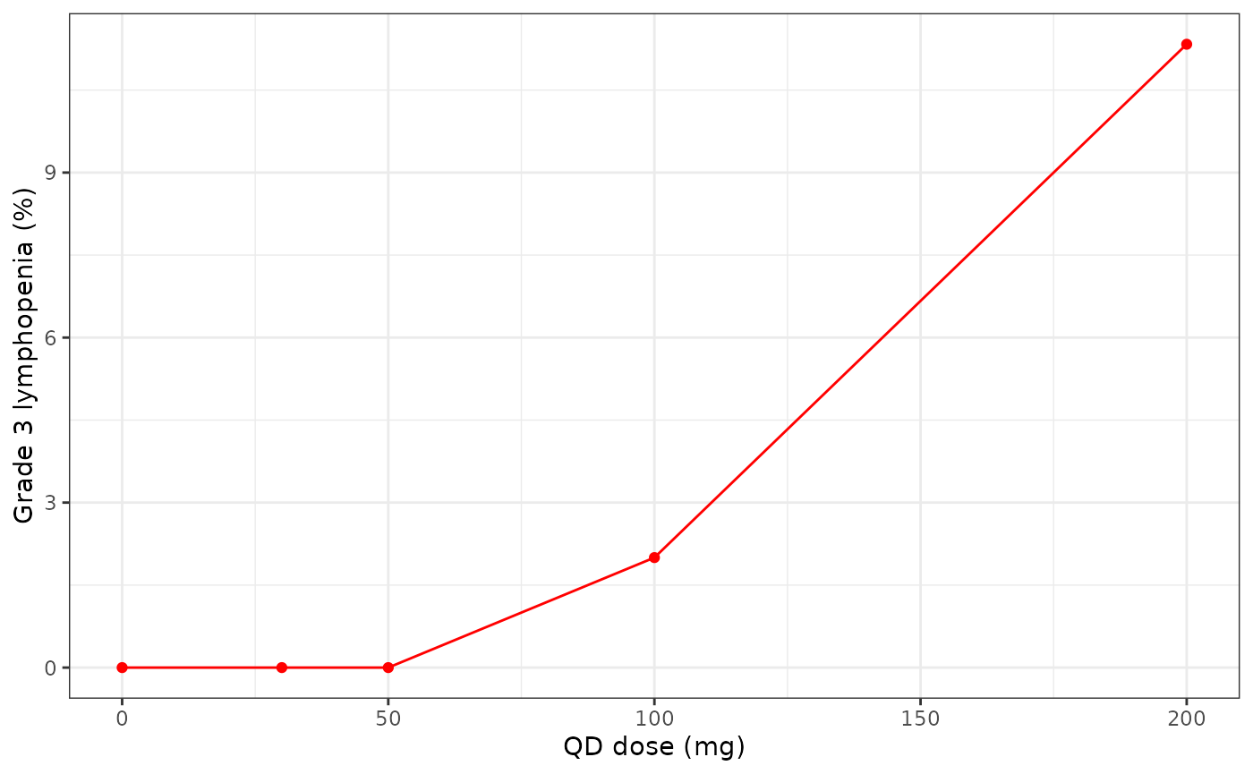
Simulated proportion of patients reaching grade 3/4 lymphopenia (nadir < 0.5 x 10^9/L, model-predicted count) within 52 weeks of QD dosing; compare the Grade 3 and Grade 4 bands of Figure 4 of Huh 2025.
Figure 4 of the paper shows a median grade 3 rate of essentially 0% up to 50 mg, under 1% at 100 mg and about 6% at 200 mg, with grade 4 near 0% throughout. The packaged model reproduces the shape (no grade 3/4 at 30-50 mg, a steep rise between 100 and 200 mg) but predicts more grade 3 events at 200 mg and a somewhat smaller relative decline at 50 mg than Table 3; see Assumptions and deviations.
Adverse-event models
With the first event only and a log(t) offset, each model’s expected count over t days is lambda = t x exp(theta0 + slope x sqrt(Cave) + covariates), and the incidence per 100 patient-years is 100 x 365.25 x exp(theta0 + slope x sqrt(Cave) + covariates) (Methods, ER Model-Based Benefit:Risk Evaluation).
ir100 <- function(lin) 100 * 365.25 * exp(lin)
inf_lin <- function(cav, asia = 0, female = 0) -9.00 - 1.31 * asia + 0.748 * female + 0.0989 * sqrt(cav)
hz_lin <- function(cav, age = 34) -11.3 + 0.0396 * (age - 34) + 0.0873 * sqrt(cav)
rash_lin <- function(cav, aa = 1, vit = 0, asia = 0, age = 34, female = 0) {
  -6.02 - 2.86 * aa - 2.73 * vit + 0.632 * asia - 0.0185 * (age - 34) + 0.521 * female +
    0.142 * sqrt(cav)
}

# The packaged models give the same lambda through rxSolve; observe a censored
# record at 365 days for a range of Cave values.
ae_ev <- tidyr::expand_grid(CAV = c(0, 27, 50, 257), SEXF = c(0, 1)) |>
  mutate(
    id = seq_len(n()), time = 365, evid = 0L, amt = 0,
    REGION_ASIA = 0, AGE = 34, DIS_ALOPECIA_AREATA = 1, DIS_VITILIGO = 0
  )
inf_sim <- rxSolve(readModelDb("Huh_2025_ritlecitinib_infections"), ae_ev, returnType = "data.frame")
rash_sim <- rxSolve(readModelDb("Huh_2025_ritlecitinib_rash"), ae_ev, returnType = "data.frame")
hz_sim <- rxSolve(readModelDb("Huh_2025_ritlecitinib_herpes_zoster"), ae_ev, returnType = "data.frame")
stopifnot(
  max(abs(inf_sim$lambda / (365 * exp(inf_lin(ae_ev$CAV, female = ae_ev$SEXF))) - 1)) < 1e-10,
  max(abs(rash_sim$lambda / (365 * exp(rash_lin(ae_ev$CAV, female = ae_ev$SEXF))) - 1)) < 1e-10,
  max(abs(hz_sim$lambda / (365 * exp(hz_lin(ae_ev$CAV))) - 1)) < 1e-10
)
30 mg versus 200 mg (Results)
The Results report that the roughly 10-fold exposure increase from 30 mg QD (geometric mean Cave 27 ng/mL) to 200 mg QD (257 ng/mL) raises the mean incidence per 100 patient-years about 3-fold for infections (11.0 to 33.2) and 4.4-fold for rash (18.3 to 80.1). The covariate mix behind the absolute values is not stated, but the ratio depends only on the slope.
ratio_tab <- data.frame(
  endpoint = c("Infections", "Rash"),
  model_ratio = c(
    exp(0.0989 * (sqrt(257) - sqrt(27))),
    exp(0.142 * (sqrt(257) - sqrt(27)))
  ),
  paper_ratio = c(33.2 / 11.0, 80.1 / 18.3)
)
ratio_tab |>
  dplyr::rename(
    "Endpoint" = endpoint,
    "Model ratio 200/30 mg" = model_ratio,
    "Huh 2025 ratio 200/30 mg" = paper_ratio
  ) |>
knitr::kable(digits = 2)| Endpoint | Model ratio 200/30 mg | Huh 2025 ratio 200/30 mg |
|---|---|---|
| Infections | 2.92 | 3.02 |
| Rash | 4.66 | 4.38 |
Covariate subgroups at 50 mg QD (Table 3)
Table 3 evaluates alopecia areata patients at 50 mg QD. The Cave used here is the typical steady-state Cave for a 68.5 kg alopecia areata patient from the embedded PK model (deterministic, so the comparison does not depend on the simulated cohort).
cav50_ev <- rbind(
  data.frame(id = 1, time = 0, amt = 50, ii = 24, addl = 13, evid = 1, cmt = "depot"),
  data.frame(id = 1, time = c(0, seq(312, 336, by = 0.05)), amt = 0, ii = 0, addl = 0,
             evid = 0, cmt = "central")
) |>
  mutate(WT = 68.5, AGE = 34, SEXF = 0, DIS_ALOPECIA_AREATA = 1)
cav50_sim <- rxSolve(rxode2::zeroRe(mod_lym), cav50_ev, maxsteps = 1e6, returnType = "data.frame") |>
  filter(time >= 312)
#> ℹ parameter labels from comments will be replaced by 'label()'
#> Warning: some etas defaulted to non-mu referenced, possible parsing error: etalcl, etalvc
#> as a work-around try putting the mu-referenced expression on a simple line
#> Warning: some etas defaulted to non-mu referenced, possible parsing error: etalcl, etalvc
#> as a work-around try putting the mu-referenced expression on a simple line
#> ℹ omega/sigma items treated as zero: 'etalcl', 'etalvc', 'etalcirc0'
cav50 <- sum(diff(cav50_sim$time) * (head(cav50_sim$Cc, -1) + tail(cav50_sim$Cc, -1)) / 2) / 24
cav50
#> [1] 52.76312

t3 <- data.frame(
  endpoint = rep(c("Infections", "Herpes zoster", "Rash"), c(3, 3, 4)),
  subgroup = c(
    "Male, non-Asia (ref)", "Female, non-Asia", "Female, Asia",
    "34 years (ref)", "15 years", "65 years",
    "Male, 34 years, non-Asia (ref)", "Female, 34 years, non-Asia",
    "Female, 15 years, non-Asia", "Female, 34 years, Asia"
  ),
  paper = c(8.71, 19.5, 5.76, 0.842, 0.421, 3.05, 13.0, 23.9, 37.4, 51.4),
  model = c(
    ir100(inf_lin(cav50)),
    ir100(inf_lin(cav50, female = 1)),
    ir100(inf_lin(cav50, female = 1, asia = 1)),
    ir100(hz_lin(cav50)),
    ir100(hz_lin(cav50, age = 15)),
    ir100(hz_lin(cav50, age = 65)),
    ir100(rash_lin(cav50)),
    ir100(rash_lin(cav50, female = 1)),
    ir100(rash_lin(cav50, female = 1, age = 15)),
    ir100(rash_lin(cav50, female = 1, asia = 1))
  )
) |>
  mutate(pct_diff = 100 * (model / paper - 1))
t3 |>
  dplyr::rename(
    "Endpoint" = endpoint,
    "Subgroup" = subgroup,
    "Huh 2025 incidence /100 PY" = paper,
    "Model incidence /100 PY" = model,
    "Difference (%)" = pct_diff
  ) |>
  knitr::kable(digits = c(0, 0, 3, 3, 1),
caption = "Replicates the adverse-event rows of Table 3 (alopecia areata, 50 mg QD).")| Endpoint | Subgroup | Huh 2025 incidence /100 PY | Model incidence /100 PY | Difference (%) |
|---|---|---|---|---|
| Infections | Male, non-Asia (ref) | 8.710 | 9.246 | 6.1 |
| Infections | Female, non-Asia | 19.500 | 19.534 | 0.2 |
| Infections | Female, Asia | 5.760 | 5.271 | -8.5 |
| Herpes zoster | 34 years (ref) | 0.842 | 0.852 | 1.2 |
| Herpes zoster | 15 years | 0.421 | 0.402 | -4.6 |
| Herpes zoster | 65 years | 3.050 | 2.908 | -4.7 |
| Rash | Male, 34 years, non-Asia (ref) | 13.000 | 14.257 | 9.7 |
| Rash | Female, 34 years, non-Asia | 23.900 | 24.004 | 0.4 |
| Rash | Female, 15 years, non-Asia | 37.400 | 34.114 | -8.8 |
| Rash | Female, 34 years, Asia | 51.400 | 45.160 | -12.1 |
stopifnot(
  # Structural: a mis-transcribed intercept or slope moves every row by tens of
  # percent.
  abs(median(t3$pct_diff)) < 10,
  max(abs(t3$pct_diff)) < 20
)
The reference rows (male, 34 years, outside Asia) agree within a few percent. The rows that switch on a covariate sit 1-14% below Table 3: the published risk ratios (for example 2.24 for female sex on infections, 2.15 for Asia on rash) are larger than the exponentiated Table 2 coefficients (exp(0.748) = 2.11, exp(0.632) = 1.88), presumably because Table 3 averages over parameter uncertainty. The model uses the Table 2 point estimates.
cav_grid <- seq(0, 600, by = 5)
fig3 <- bind_rows(
  data.frame(cav = cav_grid, endpoint = "Infections", sex = "Male", ir = ir100(inf_lin(cav_grid))),
  data.frame(cav = cav_grid, endpoint = "Infections", sex = "Female", ir = ir100(inf_lin(cav_grid, female = 1))),
  data.frame(cav = cav_grid, endpoint = "Rash", sex = "Male", ir = ir100(rash_lin(cav_grid))),
  data.frame(cav = cav_grid, endpoint = "Rash", sex = "Female", ir = ir100(rash_lin(cav_grid, female = 1)))
)
ggplot(fig3, aes(cav, ir, linetype = sex)) +
  geom_line() +
  facet_wrap(~endpoint, scales = "free_y") +
  labs(x = "Time-weighted Cave (ng/mL)", y = "Incidence per 100 patient-years", linetype = NULL) +
  theme_bw()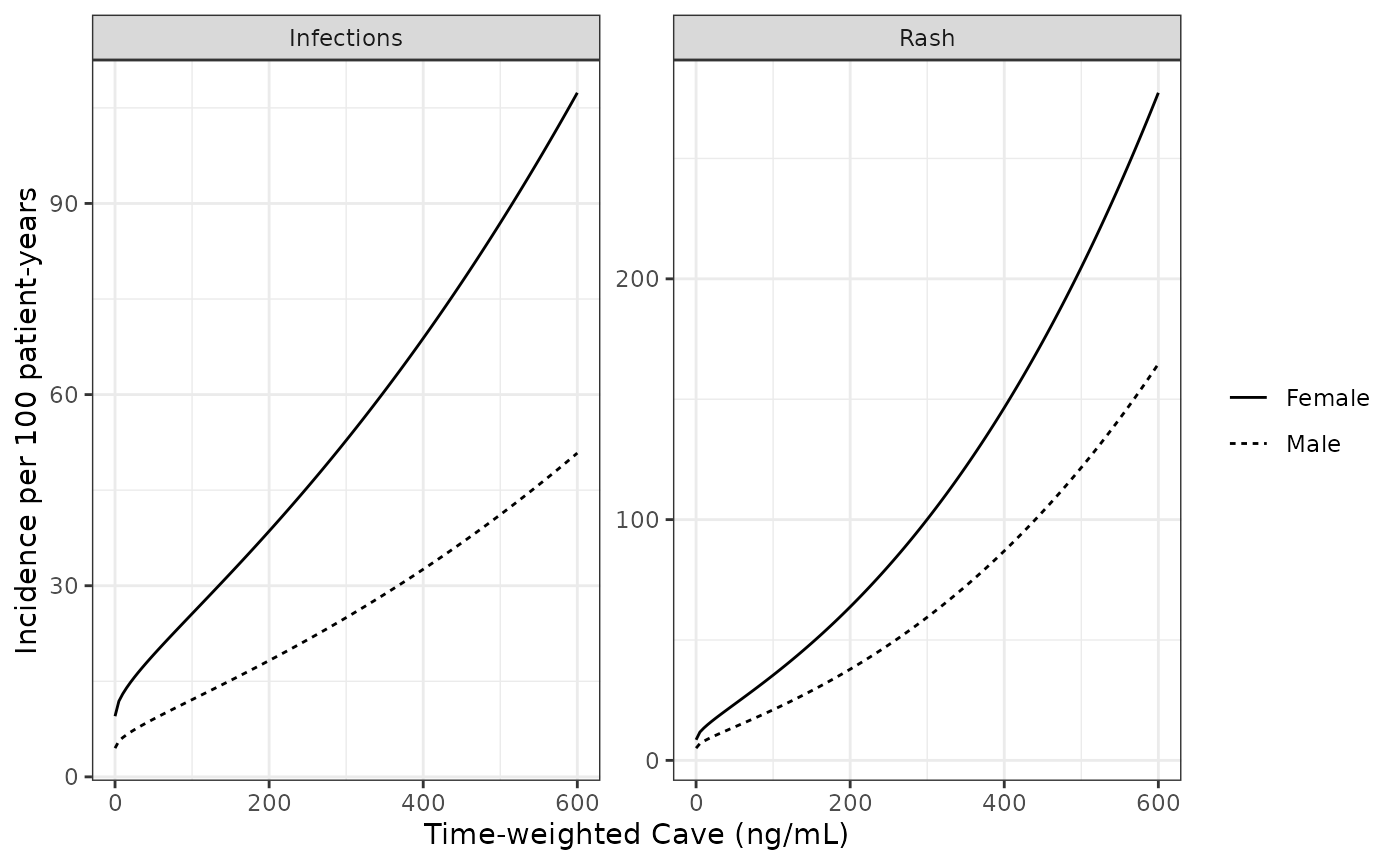
Model-predicted incidence per 100 patient-years versus time-weighted Cave for a male alopecia areata patient aged 34 years outside Asia (solid) and a female (dashed); compare the model lines of Figure 3 of Huh 2025.
Assumptions and deviations
-
C-QTc random effects read as SDs. Table 2 labels
the C-QTc random-effect rows “omega^2” and “Covariance”, but the rows
are the output of
nlme::intervals(): the slope row’s interval (2.87e-74 to 4.91e+60) is the signature of a standard deviation estimated at zero, and the “covariance” interval (-0.255 to 0.255) is symmetric and bounded the way a correlation is. The model therefore uses SD(eta0) = 4.37 ms, SD(eta1) = 3.75e-7 ms per ng/mL, correlation 5.84e-5 and residual SD 5.05 ms. Read as variances, the residual SD would be 2.2 ms, implausibly small for single QTcF readings. - C-QTc centering. The overall mean baseline QTcF is not reported; the model centers on 400 ms. The choice cancels in DeltaDeltaQTcF.
- C-QTc reference time. Table 2 lists time effects from 1 h on, so the first post-dose ECG at 0.5 h (Table 1) is the reference level carried by the intercept.
- Lymphocyte PK layer. The paper drove the lymphocyte model with empirical Bayes PK estimates from the Wojciechowski 2023 final model. For simulation the package embeds that model with all its parameters (including its IIV) fixed. Its severe-renal-impairment effect on F is omitted because the lymphocyte dataset had no renal-impairment participants. The deposited lymphocyte control stream also carries food, 800 mg and capsule effects on ka and F from the earlier PK iteration; its own comment states they do not apply to these data, and they are not carried.
- Emax normalisation. Emax = (circ0 / 1.65)^-1.6 uses the population value THETA(2), as the deposited control stream does (POPCIRC0 = THETA(2)), rather than the age- and sex-adjusted typical value. Normalising by the typical value instead gives similar lymphopenia predictions (also about 20% grade 3/4 at 200 mg in a 300-subject cohort), so this choice does not explain the differences below.
- Lymphopenia predictions versus Table 3 and Figure 4. The packaged model reproduces the Figure 2 VPC medians and the Table 3 age-group baselines, but its median relative decline at 50 mg (-11.8%, against -15.5% in the middle baseline group of Table 3) is smaller and its grade 3/4 rate at 200 mg (16%, against about 6% grade 3 and near 0% grade 4 in Figure 4) is larger. The steady-state reduction is circ0 x exp(-E / gamma) with E = Emax x Cave / EC50, so it is very sensitive to gamma and EC50 and to the simulated exposure; the paper’s simulation settings (sampled baselines, how PK variability was carried, grade evaluation on predicted or simulated counts) are not reported. The published parameters are encoded unchanged.
- Adverse-event exposure transform. Equation 3 prints a linear Cave term, but a linear term with these slopes is impossible (exp(0.0989 x 257) ~ 1e11). Supplement 2 selects among linear, square-root and log Cave by AIC, and only the square root reproduces the published 30-to-200 mg ratios, the Table 3 reference incidences and the base-model slopes of Table S2; all three models use sqrt(Cave).
- Adverse-event age effect. The Results print the herpes zoster age effect as theta0 x (Age/34)^0.0396. Applied to a negative log-scale intercept that form lowers the rate with age (65 versus 34 years gives a risk ratio of 0.75), contradicting Table 3 (3.62) and the text. Both herpes zoster and rash use the linear log-scale form theta_age x (AGE - 34), which gives 3.41 and 0.47 for 65 and 15 years (reported 3.62 and 0.500).
-
Time offset. The adverse-event models use
timeas the offset t, in days since the first dose; observation records should sit at the first event (count- or at the end of observation (count 0), with
CAVthe time-weighted average concentration up to that time.
- or at the end of observation (count 0), with
- Not packaged. The base (no covariate) first-event and recurrent-event (Poisson GEE) models of Table S2 are sensitivity analyses and are not packaged. Platelet counts were examined only descriptively (Figure S2).
- Virtual cohort. Weight and sex follow the Wojciechowski 2023 final-model population; the age mix (15% adolescents, 65% aged 18-50, 20% aged 51-72) is an assumption.
-
Solver. Year-long daily dosing with ka = 7.9 1/h
needs
maxsteps = 1e6inrxSolve().