Model and source
- Citation: Oosten AW, Abrantes JA, Jonsson S, de Bruijn P, Kuip EJM, Falcao A, van der Rijt CCD, Mathijssen RHJ. Treatment with subcutaneous and transdermal fentanyl: results from a population pharmacokinetic study in cancer patients. Eur J Clin Pharmacol. 2016 Apr;72(4):459-467. doi:10.1007/s00228-015-2005-x.
- Description: One-compartment population PK model for fentanyl administered by continuous subcutaneous infusion and transdermal matrix patch in adult cancer patients, with separate first-order absorption for each route, transdermal lag time, allometric body-weight scaling on CL/F and V/F (V/F fixed at 280 L), IIV on Ka (sc and td), F (td), and CL/F, IOV on transdermal Ka multiplexed by occasion, and proportional residual error (Oosten 2016).
- Article: https://doi.org/10.1007/s00228-015-2005-x (open access; Eur J Clin Pharmacol 2016;72(4):459-467)
Population
The model was developed from 942 fentanyl plasma samples collected in 52 adult cancer patients (3 of whom participated twice) admitted to the Erasmus MC Cancer Institute (Rotterdam, The Netherlands) between January 2010 and November 2013 for moderate-to-severe cancer-related nociceptive pain (Oosten 2016 Table 1). Median age 63 years (range 23-80); 33 male (63%), 19 female (37%); 47 (90%) Caucasian. Median body mass index was 25 kg/m^2 (range 18-40). Primary tumor sites were breast (15%), urinary tract including kidney (15%), prostate (13%), soft-tissue sarcoma / GIST (12%), colorectal (10%), and other (35%).
Subcutaneous fentanyl doses ranged from 10 to 300 ug/h continuous infusion (median 75); transdermal fentanyl Sandoz Matrix patch doses ranged from 12 to 400 ug/h (median 50), replaced every 72 h. Sampling was sparse and opportunistic: median 15 samples per patient (range 1-86), median observed concentration 1.33 ng/mL (range 0.122-10.7). 32 patients had semi- simultaneous sc and td exposure; 13 had sc samples without previous td; 9 had td samples without sc; the majority (33) already used transdermal fentanyl before admission.
The same information is available programmatically via
readModelDb("Oosten_2016_fentanyl")$population.
Source trace
Per-parameter origin is recorded as an in-file comment next to each
ini() entry in
inst/modeldb/specificDrugs/Oosten_2016_fentanyl.R. The
table below collects them for review.
| Equation / parameter | Value | Source location |
|---|---|---|
| Structural model | 1-cmt, two parallel first-order absorption depots, td lag time | Oosten 2016 Results, “Fentanyl pharmacokinetics” paragraph 1 |
lka_sc (Ka_sc) |
log(0.0358) 1/h |
Table 2: ka_sc = 0.0358 (RSE 24.4%); bootstrap 0.0374 (95% CI 0.0248-0.0555) |
lka_td (Ka_td) |
log(0.0135) 1/h |
Table 2: ka_td = 0.0135 (RSE 16.8%); bootstrap 0.0140 (95% CI 0.0105-0.0188) |
llag_td (Tlag_td) |
log(4.73) h |
Table 2: t_lag_td = 4.73 (RSE 21.2%); bootstrap 4.65 (95% CI 2.25-6.98) |
lcl (CL/F at 70 kg) |
log(49.6) L/h |
Table 2: CL_70kg/F = 49.6 (RSE 9.36%); bootstrap 50.4 (95% CI 40.9-61.6) |
lvc (V/F at 70 kg) |
fixed(log(280)) L |
Table 2 + Results: V_70kg/F fixed to 280 L (citation [25]); sensitivity-analyzed +/-50% with stable CL estimate |
lfdepot_td (F_td) |
fixed(log(1)) |
Table 2: typical F_td not separately reported; IIV only (anchor F_td = 1 at the population level) |
e_wt_cl |
fixed(0.75) |
Methods + Results: “allometrically scaled body weight on CL/F”; canonical theoretical-allometric exponent inferred |
e_wt_vc |
fixed(1) |
Methods + Results: linear weight on V/F under the same canonical-allometric inference |
etalka_sc IIV Ka_sc |
log(1 + 0.935^2) |
Table 2: IIV Ka_sc 93.5% CV (RSE 15.2%); bootstrap 91.1 (95% CI 59.6-119) |
etalka_td IIV Ka_td |
log(1 + 0.424^2) |
Table 2: IIV Ka_td 42.4% CV (RSE 23.9%); bootstrap 41.4 (95% CI 10.5-59.2) |
etalfdepot_td IIV F_td |
log(1 + 0.423^2) |
Table 2: IIV F_td 42.3% CV (RSE 30.0%); bootstrap 45.7 (95% CI 19.7-67.8) |
etalcl IIV CL/F |
log(1 + 0.432^2) |
Table 2: IIV CL/F 43.2% CV (RSE 15.2%); bootstrap 41.6 (95% CI 27.1-53.9) |
etaiov_ka_td_<n> IOV Ka_td |
log(1 + 0.328^2) (1-10) |
Table 2: IOV Ka_td 32.8% CV (RSE 51.1%); bootstrap 39.2 (95% CI 12.0-77.0); shared across occasions |
propSd |
0.234 |
Table 2: proportional residual error 23.4% CV (RSE 5.17%); bootstrap 23.2 (95% CI 20.6-25.6) |
| Concentration units | ng/mL | Methods (UPLC-MS/MS; calibration range 0.100-10.0 ng/mL); Table 2 |
| Reference subject | 70 kg adult | Table 2 footnote (CL_70kg / F and V_70kg / F headings) |
Virtual cohort
The published individual-level data are not available. The cohort below approximates the Oosten 2016 Table 1 demographics: 52 adults, 63% male / 37% female, body weight drawn from a normal distribution truncated so that the median is near 75 kg (back-computed from the published BMI median of 25 kg/m^2 at a typical adult height of 1.73 m, since individual weights are not tabulated). Every simulated subject receives the median transdermal patch dose of 50 ug/h.
set.seed(20160114) # paper online publication date
n_subj <- 52

cohort <- tibble(
  id        = seq_len(n_subj),
  WT        = pmin(pmax(rnorm(n_subj, mean = 75, sd = 14), 50), 110),
  treatment = factor("50 ug/h matrix patch")
)
The transdermal patch is parameterised as a bolus dose into the
depot2 compartment at each patch application, with
first-order release rate ka_td = 0.0135 1/h and lag time
4.73 h. The bolus amount equals the labelled patch delivery rate
multiplied by the wear time: 50 ug/h * 72 h = 3600 ug per
patch.
patch_rate_ug_h  <- 50
patch_interval_h <- 72
patch_dose_ug    <- patch_rate_ug_h * patch_interval_h # 3600 ug per patch

# Single-patch simulation to replicate Figure 1 (stochastic simulation of
# fentanyl concentrations after td 50 ug/h patch application in 52 patients).
obs_times <- sort(unique(c(seq(0, 96, by = 0.5), seq(96, 168, by = 2))))

dose_rows <- cohort |>
  dplyr::mutate(time = 0, amt = patch_dose_ug, cmt = "depot2", evid = 1L, OCC = 1L)

obs_rows <- cohort |>
  tidyr::crossing(time = obs_times) |>
  dplyr::mutate(amt = 0, cmt = NA_character_, evid = 0L, OCC = 1L)

events_td <- dplyr::bind_rows(dose_rows, obs_rows) |>
  dplyr::select(id, time, amt, cmt, evid, WT, OCC, treatment) |>
  dplyr::arrange(id, time, dplyr::desc(evid))

stopifnot(!anyDuplicated(unique(events_td[, c("id", "time", "evid")])))
Simulation
mod <- rxode2::rxode2(readModelDb("Oosten_2016_fentanyl"))
#> ℹ parameter labels from comments will be replaced by 'label()'
#> Warning: some etas defaulted to non-mu referenced, possible parsing error: etaiov_ka_td_1, etaiov_ka_td_2, etaiov_ka_td_3, etaiov_ka_td_4, etaiov_ka_td_5, etaiov_ka_td_6, etaiov_ka_td_7, etaiov_ka_td_8, etaiov_ka_td_9, etaiov_ka_td_10
#> as a work-around try putting the mu-referenced expression on a simple line
conc_unit <- mod$units[["concentration"]]
sim_td <- rxode2::rxSolve(
  mod, events = events_td,
  keep = c("WT", "treatment", "OCC")
)
Replicate published figures
Figure 1 – stochastic simulation of a 50 ug/h transdermal patch
Oosten 2016 Figure 1 shows the stochastic simulation of fentanyl plasma concentrations versus time after application of a 50 ug/h transdermal patch in 52 patients. The simulated 10-50-90 percentile envelope below should match the figure’s reported variability.
fig1 <- sim_td |>
  dplyr::filter(!is.na(Cc), time <= 168) |>
  dplyr::group_by(time, treatment) |>
  dplyr::summarise(
    Q10 = quantile(Cc, 0.10, na.rm = TRUE),
    Q50 = quantile(Cc, 0.50, na.rm = TRUE),
    Q90 = quantile(Cc, 0.90, na.rm = TRUE),
    .groups = "drop"
  )

ggplot(fig1, aes(time, Q50)) +
  geom_ribbon(aes(ymin = Q10, ymax = Q90), alpha = 0.25) +
  geom_line(linewidth = 0.7) +
  labs(x = "Time after patch application (h)",
       y = paste0("Fentanyl plasma concentration (", conc_unit, ")"),
       title = "Figure 1 -- single 50 ug/h patch, 52 simulated patients",
       caption = "Replicates Oosten 2016 Figure 1.") +
  theme_minimal()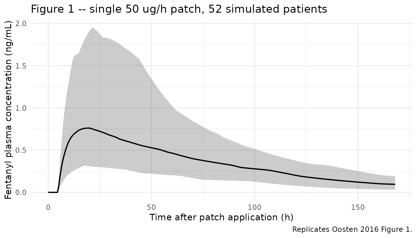
Typical-value Tmax and elimination half-life
The Oosten 2016 Discussion states that for a typical patient
receiving a transdermal patch the predicted Tmax is approximately 20.5
h, the elimination half-life is 3.91 h, and the absorption half-life is
51.3 h. The deterministic typical-value prediction below verifies these
values for a 70 kg patient receiving a single 50 ug/h patch (3600 ug
bolus into depot2).
mod_typical <- mod |> rxode2::zeroRe()
#> Warning: some etas defaulted to non-mu referenced, possible parsing error: etaiov_ka_td_1, etaiov_ka_td_2, etaiov_ka_td_3, etaiov_ka_td_4, etaiov_ka_td_5, etaiov_ka_td_6, etaiov_ka_td_7, etaiov_ka_td_8, etaiov_ka_td_9, etaiov_ka_td_10
#> as a work-around try putting the mu-referenced expression on a simple line
typical_ev <- rxode2::et(amt = patch_dose_ug, cmt = "depot2") |>
  rxode2::et(seq(0, 168, by = 0.25))
typical_ev$WT  <- 70
typical_ev$OCC <- 1L
typical_sim <- rxode2::rxSolve(mod_typical, typical_ev)
#> ℹ omega/sigma items treated as zero: 'etalka_sc', 'etalka_td', 'etalfdepot_td', 'etalcl', 'etaiov_ka_td_1', 'etaiov_ka_td_2', 'etaiov_ka_td_3', 'etaiov_ka_td_4', 'etaiov_ka_td_5', 'etaiov_ka_td_6', 'etaiov_ka_td_7', 'etaiov_ka_td_8', 'etaiov_ka_td_9', 'etaiov_ka_td_10'

# Older rxode2 versions don't always expose the residual-error endpoint Cc as
# an output column after zeroRe(); fall back to central/Vc directly. Vc at the
# reference 70 kg is 280 L (lvc <- fixed(log(280)), e_wt_vc = 1, WT = 70).
cc_vec <- if (!is.null(typical_sim$Cc)) typical_sim$Cc else typical_sim$central / 280
finite_idx <- which(is.finite(cc_vec))
if (length(finite_idx) > 0L) {
  peak_idx  <- finite_idx[which.max(cc_vec[finite_idx])]
  tmax_h    <- typical_sim$time[peak_idx]
  cmax_ngmL <- cc_vec[peak_idx]
} else {
  tmax_h    <- NA_real_
  cmax_ngmL <- NA_real_
}
thalf_el  <- log(2) * 280 / 49.6  # ln(2) * V/CL at 70 kg
thalf_a   <- log(2) / 0.0135       # td absorption half-life

knitr::kable(tibble::tibble(
  Quantity = c("Tmax (h)", "Cmax (ng/mL)", "Elimination half-life (h)",
               "Transdermal absorption half-life (h)"),
  Predicted = c(sprintf("%.1f", tmax_h),
                sprintf("%.3f", cmax_ngmL),
                sprintf("%.2f", thalf_el),
                sprintf("%.1f", thalf_a)),
  `Oosten 2016 reported` = c("~20.5 (Discussion)", "Not directly tabulated",
                             "3.91 (Discussion)", "51.3 (Discussion)")
), caption = "Typical-value verification for a 70 kg adult, single 50 ug/h td patch.")| Quantity | Predicted | Oosten 2016 reported |
|---|---|---|
| Tmax (h) | 20.5 | ~20.5 (Discussion) |
| Cmax (ng/mL) | 0.792 | Not directly tabulated |
| Elimination half-life (h) | 3.91 | 3.91 (Discussion) |
| Transdermal absorption half-life (h) | 51.3 | 51.3 (Discussion) |
Figure 4 – rotation from sc 50 ug/h to a td 50 ug/h patch (12-h scheme)
Oosten 2016 Figure 4 simulates plasma fentanyl during rotation from a sc infusion of 50 ug/h at steady state to a td patch with delivery rate 50 ug/h using the 12-h scheme: after patch application, sc is continued at 100% for 6 h, then tapered to 50% for the next 6 h, then stopped.
# Steady-state sc infusion before rotation (start at -240 h so by t = 0 the
# system is at sc steady state; 240 h is roughly 60 * sc absorption half-life
# of 19.4 h, plenty for equilibration).
ss_h    <- 240
sc_rate <- 50  # ug/h

cohort_rot <- tibble(
  id        = seq_len(n_subj),
  WT        = pmin(pmax(rnorm(n_subj, mean = 75, sd = 14), 50), 110),
  treatment = factor("Rotation 12-h scheme")
)

# Rotation dose schedule, all times in absolute hours from rotation time = 0.
# sc piecewise rates: 50 ug/h for [-ss_h, +6); 25 ug/h for [+6, +12); 0 thereafter.
# td patch (3600 ug bolus to depot2 with OCC = 1) at t = 0.
sc_phase1 <- cohort_rot |>
  dplyr::mutate(time = -ss_h, amt = sc_rate * (ss_h + 6),
                rate = sc_rate, cmt = "depot", evid = 1L, OCC = 0L)
sc_phase2 <- cohort_rot |>
  dplyr::mutate(time = 6, amt = (sc_rate / 2) * 6,
                rate = sc_rate / 2, cmt = "depot", evid = 1L, OCC = 0L)
td_patch <- cohort_rot |>
  dplyr::mutate(time = 0, amt = patch_dose_ug,
                rate = NA_real_, cmt = "depot2", evid = 1L, OCC = 1L)

rot_obs_times <- sort(unique(c(seq(-24, 96, by = 1))))
obs_rot <- cohort_rot |>
  tidyr::crossing(time = rot_obs_times) |>
  dplyr::mutate(amt = 0, rate = NA_real_, cmt = NA_character_,
                evid = 0L, OCC = 1L)

events_rot <- dplyr::bind_rows(sc_phase1, sc_phase2, td_patch, obs_rot) |>
  dplyr::select(id, time, amt, rate, cmt, evid, WT, OCC, treatment) |>
  dplyr::arrange(id, time, dplyr::desc(evid))

stopifnot(!anyDuplicated(unique(events_rot[, c("id", "time", "evid")])))

sim_rot <- rxode2::rxSolve(mod, events = events_rot,
                           keep = c("WT", "treatment", "OCC"))
#> Warning:
#> with negative times, compartments initialize at first negative observed time
#> with positive times, compartments initialize at time zero
#> use 'rxSetIni0(FALSE)' to initialize at first observed time
#> this warning is displayed once per session
fig4 <- sim_rot |>
  dplyr::filter(!is.na(Cc), time >= -24, time <= 96) |>
  dplyr::group_by(time) |>
  dplyr::summarise(
    Q10 = quantile(Cc, 0.10, na.rm = TRUE),
    Q50 = quantile(Cc, 0.50, na.rm = TRUE),
    Q90 = quantile(Cc, 0.90, na.rm = TRUE),
    .groups = "drop"
  )

ggplot(fig4, aes(time, Q50)) +
  geom_ribbon(aes(ymin = Q10, ymax = Q90), alpha = 0.25) +
  geom_line(linewidth = 0.7) +
  geom_vline(xintercept = 0, linetype = "dashed", colour = "grey60") +
  labs(x = "Time relative to patch application (h)",
       y = paste0("Fentanyl plasma concentration (", conc_unit, ")"),
       title = "Figure 4 -- sc 50 ug/h -> td 50 ug/h rotation, 12-h scheme",
       caption = "Replicates Oosten 2016 Figure 4. Dashed line = patch application time.") +
  theme_minimal()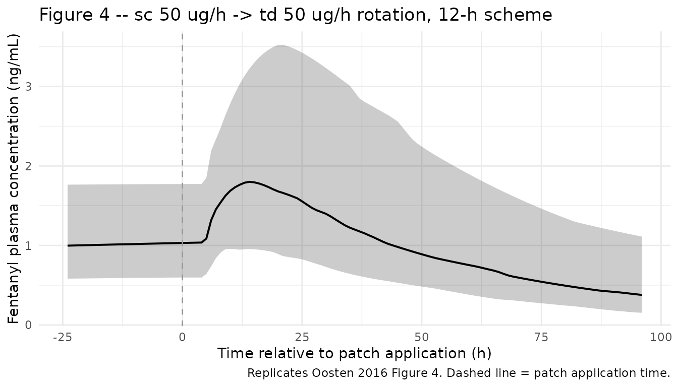
Oosten 2016 reports for this rotation scheme that 12 h after patch application the 10th and 90th percentiles are 0.87 and 3.22 ng/mL respectively, with a median of 1.68 ng/mL. The simulated values below should be within sampling noise of these.
rot_12h <- sim_rot |>
  dplyr::filter(time == 12) |>
  dplyr::summarise(
    Q10 = quantile(Cc, 0.10, na.rm = TRUE),
    median = quantile(Cc, 0.50, na.rm = TRUE),
    Q90 = quantile(Cc, 0.90, na.rm = TRUE)
  )

knitr::kable(tibble::tibble(
  Percentile = c("10th", "Median", "90th"),
  Simulated = sprintf("%.2f", c(rot_12h$Q10, rot_12h$median, rot_12h$Q90)),
  `Oosten 2016 Figure 4 caption / Results` = c("0.87", "1.68", "3.22")
), caption = "Plasma concentration 12 h after patch application (rotation 12-h scheme).")| Percentile | Simulated | Oosten 2016 Figure 4 caption / Results |
|---|---|---|
| 10th | 0.90 | 0.87 |
| Median | 1.46 | 1.68 |
| 90th | 2.68 | 3.22 |
PKNCA validation
PKNCA single-dose NCA over the 168 h post-patch window for the
stochastic td-only cohort. The treatment grouping comes before
id in the formula per project convention. Half-life is
computed from the declining post-Cmax phase, which under the
slow-absorption / fast- elimination regime reflects absorption rather
than elimination (flip-flop kinetics, Oosten 2016
Discussion).
sim_nca <- sim_td |>
  dplyr::filter(!is.na(Cc)) |>
  dplyr::select(id, time, Cc, treatment)

dose_df <- events_td |>
  dplyr::filter(evid == 1) |>
  dplyr::select(id, time, amt, treatment)

conc_obj <- PKNCA::PKNCAconc(sim_nca, Cc ~ time | treatment + id,
                             concu = "ng/mL", timeu = "h")
dose_obj <- PKNCA::PKNCAdose(dose_df, amt ~ time | treatment + id,
                             doseu = "ug")

intervals <- data.frame(
  start      = 0,
  end        = 168,
  cmax       = TRUE,
  tmax       = TRUE,
  auclast    = TRUE,
  half.life  = TRUE
)

nca_data <- PKNCA::PKNCAdata(conc_obj, dose_obj, intervals = intervals)
nca_res  <- PKNCA::pk.nca(nca_data)
knitr::kable(summary(nca_res),
caption = "Single-dose NCA over 168 h post-patch (50 ug/h Durogesic matrix, n = 52).")| Interval Start | Interval End | treatment | N | AUClast (h*ng/mL) | Cmax (ng/mL) | Tmax (h) | Half-life (h) |
|---|---|---|---|---|---|---|---|
| 0 | 168 | 50 ug/h matrix patch | 52 | 54.5 [54.8] | 0.700 [77.4] | 19.5 [12.5, 35.0] | 63.4 [39.2] |
Assumptions and deviations
-
Allometric exponents inferred at canonical values.
Oosten 2016 states “allometrically scaled body weight on CL/F and V/F
was found to explain some variability and was kept to increase model
stability” (Results, Fentanyl pharmacokinetics) but does not numerically
list the exponents. The library model uses the canonical
theoretical-allometric values 0.75 on CL/F and 1.0 on V/F because (a)
the Table 2 headings “CL_70kg / F” and “V_70kg / F” imply a
(WT / 70 kg)normalization consistent with the canonical idiom; (b) the paper does not estimate or report alternative exponents; and (c) V/F is fixed in the structural model, so any custom exponent on V/F would not change the V/F estimate. Encoded withfixed(0.75)andfixed(1)so users see the assumption. -
V/F fixed. V/F was fixed to 280 L/70 kg in the
paper (Oosten 2016 Table 2 + Results citation [25]) because the
sparse-sampling design did not support estimation of all absorption +
disposition parameters; a sensitivity analysis varying V/F by +/-50% in
10% increments showed the model insensitive to the value, with only
Tlag_td and Ka_sc varying slightly. The library model preserves V/F =
280 L/70 kg as
fixed(). -
F_td anchored at 1 at the population level. Oosten
2016 Table 2 lists only the IIV on F_td (42.3% CV) without a separately
tabulated typical value. The library model encodes the typical F_td as
fixed(log(1))and allows the IIV around that anchor; the reference subcutaneous route has its bioavailability implicitly anchored at 1 by leavingf(depot)unset. This is the conventional popPK convention for a reference route – the model is parameterised in apparent clearance (CL/F) and apparent volume (V/F), so absolute bioavailability is unidentifiable without an absolute reference dose. -
IOV multiplexed to 10 transdermal occasions. Oosten
2016 defines an occasion as “a transdermal dose followed by at least one
observation” and the patient cohort had a variable number of patch
occasions; the library model encodes the per-occasion IOV variance via a
fixed set of ten occasion-indicator etas (
etaiov_ka_td_1..etaiov_ka_td_10), with the variance estimated for occasion 1 andfix()-ed equal across occasions 2..10 (NONMEM$OMEGA BLOCK(1) SAMEtranslation). The cap reflects typical hospital-stay simulations: patches change every 72 h so 10 occasions span a 30-day window. Records withOCCoutside 1..10 zero every indicator and yield the typical-value Ka_td (no IOV applied), which is appropriate for non-transdermal records and for simulations beyond ten patch occasions. Users who need more occasions can extend the IOV block. -
Residual error: “additive on the log-scale” ->
proportional. The paper’s parameterization in NONMEM treats
epsas additive on the log-transformed concentration; this maps cleanly to a proportional error model in nlmixr2’s linear-concentration space for small-to- moderate CV (here 23.4%), and that is the encoding used. - Race / ethnicity neutral cohort. Race is reported in Oosten 2016 Table 1 (90% Caucasian, 2% other, 8% unknown) but is not a model covariate; the simulated cohort is neutral on race.
- Weight distribution. Individual body weights were not tabulated in Oosten 2016; only the median BMI of 25 kg/m^2 was reported (range 18-40). The vignette samples body weight from a normal distribution centred at 75 kg (back-computed from the BMI median at 1.73 m typical height) with SD 14 kg, truncated to [50, 110] kg. Users with their own trial cohort should override the cohort generation.
-
Units alignment. Dosing is parameterised in
micrograms (
ug) and concentration inng/mL. Because1 ug / 1 L = 1 ng/mL, no explicit scaling factor is needed inmodel();checkModelConventions()surfaces aninfoflag noting the apparent numerator difference but the units are dimensionally consistent.