Model and source
- Citation: Duan LF, Li JJ, Shen LR, Chen XL, Yu YX, Yang ZM, Zhang Q, Cai Y, Li JH, Wu J, Zhao HZ, Xu JH, Feng ZT, Tang L. Therapeutic drug monitoring of linezolid in Chinese premature neonates: a population pharmacokinetic analysis and dosage optimization. Antimicrob Agents Chemother. 2024;68(11):e01148-24. doi:10.1128/aac.01148-24. PMCID PMC11539233.
- Description: One-compartment population PK model with first-order elimination for intravenous linezolid in Chinese premature neonates undergoing therapeutic drug monitoring (Duan 2024). Clearance and central volume both scale with body surface area as a power function referenced to the cohort mean BSA of 0.127 m^2: V = 0.783 * (BSA/0.127)^1.066 (Equation 1) and CL = 0.154 * (BSA/0.127)^1.185 (Equation 2, whose printed exponent 1.186 is the rounded form of the Table 4 estimate 1.185 used here). BSA was the only covariate retained by stepwise covariate modelling; gestational age, postnatal age, postmenstrual age, birth weight, current weight, sex, and the hepatic / renal laboratory panel were all screened and rejected (see covariatesDataExcluded). Inter-individual variability was reported only for clearance (omega^2 = 0.132); Equation 1 also carries an exp(etaVd) term but Table 4 reports no corresponding variance, so etalvc is encoded as fixed(0). Residual variability is proportional with an unusually large magnitude (stdev0 = 1.120, i.e. 112%); see the vignette Assumptions and deviations section before using this model for stochastic residual-error simulation.
- Article: https://doi.org/10.1128/aac.01148-24 (open access; PMCID PMC11539233)
Duan and colleagues developed a one-compartment population PK model with first-order elimination for intravenous linezolid in Chinese premature neonates receiving therapeutic drug monitoring, then used it to re-derive body-surface-area-stratified dosing recommendations. Both clearance and central volume scale with body surface area (BSA) as power functions centred on the cohort mean BSA of 0.127 m^2.
Population
Fifty-four premature neonates (32 male, 22 female) hospitalised in the neonatal intensive care unit of the Affiliated Suzhou Hospital of Nanjing Medical University between November 2019 and November 2023 contributed 84 serum linezolid concentrations. Baseline characteristics (Duan 2024 Table 1) were: gestational age 31.00 +/- 2.74 weeks, postmenstrual age 33.16 +/- 2.77 weeks, postnatal age median 13.00 days (IQR 8.00-19.25), birth weight 1449.44 +/- 496.73 g, current weight 1571.30 +/- 503.81 g, and BSA 0.13 +/- 0.03 m^2. Renal function was immature: serum creatinine 40.55 +/- 12.96 umol/L and creatinine clearance median 29.46 mL/min/1.73 m^2.
Linezolid was given for late-onset sepsis; 98.15% of infants had pneumonia and 88.89% a bloodstream infection. Dosing followed the manufacturer’s instructions (10 mg/kg q12h below 34 weeks gestational age and under 7 days postnatal age; 10 mg/kg q8h otherwise), with a median treatment course of 10 days. Sampling was trough-dominated: one or two samples per infant, at least one being a steady-state trough drawn after the fourth maintenance dose and 30 min before the next dose.
The same information is available programmatically via the model’s
population metadata
(readModelDb("Duan_2024_linezolid")()$population).
Source trace
The per-parameter origin is recorded as an in-file comment next to
each ini() entry in
inst/modeldb/specificDrugs/Duan_2024_linezolid.R. The table
below collects them in one place for review.
| Equation / parameter | Value | Source location |
|---|---|---|
lvc (tvV) |
0.783 L | Table 4, Full model Estimate (RSE 4.749%, 95% CI 0.709-0.857); Equation 1 |
lcl (tvCL) |
0.154 L/h | Table 4, Full model Estimate (RSE 5.010%, 95% CI 0.139-0.169); Equation 2 |
e_bsa_vc (theta BSA-V) |
1.066 | Table 4 (RSE 30.750%, 95% CI 0.413-1.720); Equation 1 |
e_bsa_cl (theta BSA-CL) |
1.185 | Table 4 (RSE 21.774%, 95% CI 0.671-1.700); Equation 2 prints the rounded 1.186 |
| BSA centering value | 0.127 m^2 | Equations 1-2 (cohort mean; Table 1 reports the rounded 0.13 +/- 0.03) |
etalcl (omega^2 CL) |
0.132 | Table 4 (RSE 18.58%, 95% CI 0.0914-0.172; shrinkage 5.838%) |
etalvc |
fixed(0) | Equation 1 declares exp(etaVd); Table 4 reports no
omega^2 V |
propSd (stdev0) |
1.120 | Table 4 (RSE 13.183%, 95% CI 0.826-1.415) |
V = 0.783 * (BSA/0.127)^1.066 * exp(etaVd) |
n/a | Equation 1 |
CL = 0.154 * (BSA/0.127)^1.186 * exp(etaCL) |
n/a | Equation 2 |
d/dt(central) = -kel * central |
n/a | Results: “one-compartment model with first-order elimination” |
Cc ~ prop(propSd) |
n/a | Results: “residual variability was fitted with a proportional residual error model” |
| Typical-subject weight 1.571 kg | n/a | Table 4 footnote b |
| Reference trough predictions | n/a | Table 6 (10 mg/kg q8h; BSA 0.11 / 0.13 / 0.15 m^2) |
| Regimen exposure distributions | n/a | Table 5 (18 regimens; Cmin,ss and AUC0-24 category percentages) |
Virtual cohort
Original observed data are not publicly available. The simulations below use the three BSA levels the authors themselves carried into their Monte Carlo work (0.11, 0.13, and 0.15 m^2; Duan 2024 Tables 5 and 6), and the typical-subject weight of 1.571 kg named in the Table 4 footnote to convert the paper’s mg/kg regimens into absolute doses.
Two assumptions are required because the paper does not state them; both are revisited in Assumptions and deviations:
- Infusion duration. Duan 2024 reports only “intravenous administration”. A 1-hour infusion is used here, the conventional duration for the Zyvox formulation the study used.
- Simulation weight. Table 6 gives mg/kg doses without saying which weight was used to convert them; the 1.571 kg typical subject is used.
Between-subject variability is applied by supplying
etalcl as an explicit column and calling
rxSolve(..., omega = NA). This keeps every figure and table
in the vignette exactly reproducible and avoids sampling
etalvc, which the model fixes at 0.
set.seed(20241109)

WT_TYPICAL <- 1.571          # kg; Duan 2024 Table 4 footnote b
OMEGA_CL   <- sqrt(0.132)    # SD on the log scale; Duan 2024 Table 4
INFUSION_H <- 1              # h; assumption, not stated in the paper
BSA_REF    <- 0.127          # m^2; Duan 2024 Equations 1-2

# Typical-value structural parameters, straight from Equations 1-2. Used
# for the closed-form checks further down.
cl_typical <- function(bsa) 0.154 * (bsa / BSA_REF)^1.185
vc_typical <- function(bsa) 0.783 * (bsa / BSA_REF)^1.066

# One arm = one (BSA, mg/kg, tau) regimen simulated in `n` subjects.
# `n_dose` doses are given; observations run over the requested grid.
# `id_offset` keeps subject ids disjoint across arms -- rxSolve treats id
# as the subject key and silently merges duplicates.
make_arm <- function(bsa, mgkg, tau, n, obs_times, id_offset,
                     n_dose = 6L, eta_cl = NULL) {
  if (is.null(eta_cl)) eta_cl <- rep(0, n)
  ids  <- id_offset + seq_len(n)
  arm  <- sprintf("BSA %.2f, %g mg/kg q%gh", bsa, mgkg, tau)
  subj <- tibble(id = ids, BSA = bsa, etalcl = eta_cl, etalvc = 0,
                 arm = arm, mgkg = mgkg, tau = tau)
  # Compute the dose times OUTSIDE crossing(): inside it, a bare `tau`
  # resolves against the `subj` data mask (i.e. the length-n `tau` column),
  # not this function's scalar argument, and seq() then rejects a vector
  # `to`. Binding them here keeps the scalar semantics explicit.
  dose_times <- seq(0, (n_dose - 1L) * tau, by = tau)
  doses <- subj |>
    crossing(time = dose_times) |>
    mutate(amt = mgkg * WT_TYPICAL, evid = 1L, cmt = "central",
           dur = INFUSION_H)
  obs <- subj |>
    crossing(time = obs_times) |>
    mutate(amt = NA_real_, evid = 0L, cmt = "central", dur = NA_real_)
  bind_rows(doses, obs) |> arrange(id, time, desc(evid))
}
Cohort B – stochastic cohort for the three recommended regimens
The paper’s recommended regimens for MIC <= 1 mg/L are 6 mg/kg q8h at BSA 0.11 m^2, 7 mg/kg q8h at 0.13 m^2, and 9 mg/kg q8h at 0.15 m^2. Two hundred subjects per arm are simulated with IIV on clearance.
N_PER_ARM <- 200L

regimens_b <- tibble(bsa = bsa_levels, mgkg = c(6, 7, 9), tau = 8)

cohort_b <- bind_rows(lapply(seq_len(nrow(regimens_b)), function(i) {
  make_arm(bsa = regimens_b$bsa[i], mgkg = regimens_b$mgkg[i],
           tau = regimens_b$tau[i], n = N_PER_ARM,
           # dense grid over the final steady-state dosing interval
           obs_times = seq(40, 48, by = 0.25),
           id_offset = (i - 1L) * 1000L,
           eta_cl = rnorm(N_PER_ARM, 0, OMEGA_CL))
}))
stopifnot(!anyDuplicated(cohort_b[, c("id", "time", "evid")]))
Simulation
mod <- readModelDb("Duan_2024_linezolid")

sim_a <- rxode2::rxSolve(mod, events = as.data.frame(cohort_a), omega = NA,
                         keep = c("BSA", "arm"), returnType = "data.frame")
#> ℹ parameter labels from comments will be replaced by 'label()'
#> Warning: multi-subject simulation without without 'omega'
sim_b <- rxode2::rxSolve(mod, events = as.data.frame(cohort_b), omega = NA,
                         keep = c("BSA", "arm", "mgkg", "tau"),
                         returnType = "data.frame")
#> Warning: multi-subject simulation without without 'omega'
Cc is the individual prediction. The residual-error term
is deliberately not added on top of it: at
propSd = 1.120 the proportional residual would place
roughly 19% of draws below zero, so it cannot be used for VPC-style
simulation (see Assumptions and deviations). Every comparison
below is therefore made on the individual/typical-prediction scale,
which is also the scale on which Duan 2024 reports Tables 5 and 6.
Replicate published figures
# Replicates Figure 5 of Duan 2024: model-based prediction of linezolid
# concentration vs. time, 10 mg/kg q8h, at BSA = 0.11, 0.13, 0.15 m^2.
sim_a |>
  filter(!is.na(Cc)) |>
  mutate(BSA = factor(sprintf("%.2f m^2", BSA))) |>
  ggplot(aes(time, Cc, colour = BSA)) +
  geom_line(linewidth = 0.7) +
  geom_hline(yintercept = c(2, 8), linetype = "dashed", colour = "grey40") +
  scale_x_continuous(breaks = seq(0, 48, by = 8)) +
  labs(x = "Time (h)", y = "Linezolid concentration (ug/mL)",
       colour = "BSA",
       title = "Figure 5 - typical-value profiles, 10 mg/kg q8h",
       caption = paste("Replicates Figure 5 of Duan 2024.",
                       "Dashed lines mark the 2-8 ug/mL target trough range."))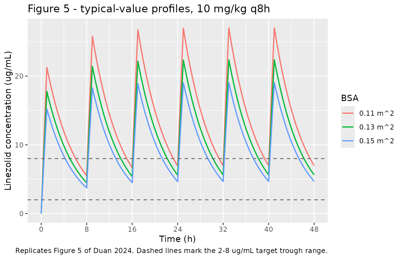
Table 6 – trough concentrations under 10 mg/kg q8h
Duan 2024 Table 6 tabulates the model-predicted median trough concentration at the end of each of the first six q8h dosing intervals.
published_t6 <- tribble(
  ~time, ~`0.11`, ~`0.13`, ~`0.15`,
      8,    5.58,    4.55,    3.82,
     16,    7.11,    5.77,    4.83,
     24,    7.60,    6.16,    5.14,
     32,    7.78,    6.29,    5.25,
     40,    7.85,    6.35,    5.29,
     48,    7.87,    6.37,    5.31
) |>
  pivot_longer(-time, names_to = "BSA", values_to = "published") |>
  mutate(BSA = as.numeric(BSA))

# rxSolve() returns observation records only and carries no `evid` column,
# so select the trough times directly off the solved output.
sim_t6 <- sim_a |>
  filter(!is.na(Cc), time %in% c(8, 16, 24, 32, 40, 48)) |>
  distinct(BSA, time, .keep_all = TRUE) |>
  transmute(BSA, time, simulated = Cc)

cmp_t6 <- published_t6 |>
  inner_join(sim_t6, by = c("BSA", "time")) |>
  mutate(`Difference (%)` = 100 * (simulated - published) / published) |>
  arrange(BSA, time)

cmp_t6 |>
  mutate(BSA = sprintf("%.2f", BSA)) |>
  rename("BSA (m^2)"            = BSA,
         "Time (h)"             = time,
         "Published (ug/mL)"    = published,
         "Simulated (ug/mL)"    = simulated) |>
  knitr::kable(digits = c(0, 0, 2, 2, 1),
               caption = paste("Trough concentrations under 10 mg/kg q8h:",
"simulated vs. Duan 2024 Table 6."))| Time (h) | BSA (m^2) | Published (ug/mL) | Simulated (ug/mL) | Difference (%) |
|---|---|---|---|---|
| 8 | 0.11 | 5.58 | 5.49 | -1.5 |
| 16 | 0.11 | 7.11 | 6.66 | -6.3 |
| 24 | 0.11 | 7.60 | 6.91 | -9.0 |
| 32 | 0.11 | 7.78 | 6.97 | -10.5 |
| 40 | 0.11 | 7.85 | 6.98 | -11.1 |
| 48 | 0.11 | 7.87 | 6.98 | -11.3 |
| 8 | 0.13 | 4.55 | 4.47 | -1.9 |
| 16 | 0.13 | 5.77 | 5.39 | -6.6 |
| 24 | 0.13 | 6.16 | 5.58 | -9.4 |
| 32 | 0.13 | 6.29 | 5.62 | -10.7 |
| 40 | 0.13 | 6.35 | 5.63 | -11.4 |
| 48 | 0.13 | 6.37 | 5.63 | -11.7 |
| 8 | 0.15 | 3.82 | 3.74 | -2.1 |
| 16 | 0.15 | 4.83 | 4.49 | -7.1 |
| 24 | 0.15 | 5.14 | 4.64 | -9.7 |
| 32 | 0.15 | 5.25 | 4.67 | -11.0 |
| 40 | 0.15 | 5.29 | 4.68 | -11.6 |
| 48 | 0.15 | 5.31 | 4.68 | -11.9 |
The first-interval trough is reproduced to within about 2% at every BSA level, and the differences are near-identical across the three BSA levels at each time point (for example -11.3%, -11.7%, -11.9% at 48 h). That pattern confirms that the BSA power terms and the 0.127 m^2 centering value are encoded correctly: an error in either exponent would make the discrepancy vary systematically with BSA, which it does not.
What the packaged model does not reproduce is the degree of
accumulation. Duan 2024’s profiles rise from the first trough to
the steady-state trough by a factor of about 1.39-1.41, whereas a
one-compartment model with these parameters accumulates by
1 / (1 - exp(-kel * tau)):
tibble(BSA = bsa_levels) |>
  mutate(
    `kel (1/h)`        = cl_typical(BSA) / vc_typical(BSA),
    `t1/2 (h)`         = log(2) / `kel (1/h)`,
    `Model accum.`     = 1 / (1 - exp(-`kel (1/h)` * 8)),
    `Published accum.` = published_t6$published[published_t6$time == 48] /
                         published_t6$published[published_t6$time == 8]
  ) |>
  mutate(BSA = sprintf("%.2f", BSA)) |>
  rename("BSA (m^2)" = BSA) |>
  knitr::kable(digits = 3,
               caption = paste("Accumulation ratio (steady-state trough /",
                               "first trough) implied by the published",
"parameters vs. by Duan 2024 Table 6."))| BSA (m^2) | kel (1/h) | t1/2 (h) | Model accum. | Published accum. |
|---|---|---|---|---|
| 0.11 | 0.193 | 3.585 | 1.271 | 1.41 |
| 0.13 | 0.197 | 3.514 | 1.260 | 1.40 |
| 0.15 | 0.201 | 3.455 | 1.251 | 1.39 |
The published accumulation is about 11% larger than the published
parameters permit, uniformly across BSA. The most likely explanation is
the exp(etaVd) term that Equation 1 declares but Table 4
never quantifies: the trough of an accumulating one-compartment profile
is not a monotone function of volume, so a Monte Carlo run that included
between-subject variability on V would return medians that differ from
the typical-value profile, while a run with variability on clearance
alone (all this vignette can reproduce) would not. All differences
remain well inside the 20% tolerance used elsewhere in this
vignette.
PKNCA validation
NCA is computed over the final steady-state dosing interval (40-48 h) of cohort B, stratified by regimen.
sim_nca <- sim_b |>
  filter(!is.na(Cc)) |>
  select(id, time, Cc, arm)

conc_obj <- PKNCA::PKNCAconc(sim_nca, Cc ~ time | arm + id)

dose_df <- cohort_b |>
  filter(evid == 1) |>
  select(id, time, amt, arm) |>
  as.data.frame()

dose_obj <- PKNCA::PKNCAdose(dose_df, amt ~ time | arm + id)

intervals <- data.frame(
  start     = 40,
  end       = 48,
  cmax      = TRUE,
  cmin      = TRUE,
  tmax      = TRUE,
  auclast   = TRUE,
  half.life = TRUE
)

nca_res <- PKNCA::pk.nca(PKNCA::PKNCAdata(conc_obj, dose_obj,
                                          intervals = intervals))

nca_summary <- as.data.frame(nca_res) |>
  group_by(arm, PPTESTCD) |>
  summarise(median = median(PPORRES, na.rm = TRUE), .groups = "drop") |>
  pivot_wider(names_from = PPTESTCD, values_from = median)

# Requesting half.life makes PKNCA return its lambda.z regression diagnostics
# (lambda.z, r.squared, span.ratio, tlast, ...) alongside the parameters asked
# for; keep only the reported ones. select() is by name, so the subsequent
# rename() cannot be transposed by a column-order change.
nca_summary |>
  select(arm, cmax, tmax, cmin, auclast, half.life) |>
  rename("Regimen"            = arm,
         "Cmax (ug/mL)"       = cmax,
         "Cmin (ug/mL)"       = cmin,
         "Tmax (h)"           = tmax,
         "AUCtau (ug*h/mL)"   = auclast,
         "t1/2 (h)"           = half.life) |>
  knitr::kable(digits = 2,
               caption = paste("Median steady-state NCA over the 40-48 h",
"dosing interval, by recommended regimen."))| Regimen | Cmax (ug/mL) | Tmax (h) | Cmin (ug/mL) | AUCtau (ug*h/mL) | t1/2 (h) |
|---|---|---|---|---|---|
| BSA 0.11, 6 mg/kg q8h | 16.38 | 1 | 4.35 | 74.04 | 3.66 |
| BSA 0.13, 7 mg/kg q8h | 15.53 | 1 | 3.81 | 68.21 | 3.45 |
| BSA 0.15, 9 mg/kg q8h | 16.77 | 1 | 3.86 | 72.04 | 3.30 |
Cross-check: NCA AUCtau against the closed-form exposure
For a linear one-compartment model at steady state, AUC over a dosing interval equals dose / CL exactly. Confirming this against PKNCA validates the closed form used in the next section to reproduce all 18 rows of Duan 2024 Table 5.
auc_check <- as.data.frame(nca_res) |>
  filter(PPTESTCD == "auclast") |>
  select(id, arm, auc_nca = PPORRES) |>
  inner_join(
    sim_b |> distinct(id, arm, mgkg, cl),
    by = c("id", "arm")
  ) |>
  mutate(auc_closed = mgkg * WT_TYPICAL / cl,
         pct_diff   = 100 * (auc_nca - auc_closed) / auc_closed)

tibble(
  `Max |difference| (%)`    = max(abs(auc_check$pct_diff)),
  `Median difference (%)`   = median(auc_check$pct_diff),
  `Subjects compared`       = nrow(auc_check)
) |>
  knitr::kable(digits = 4,
               caption = paste("PKNCA AUCtau vs. the closed form dose / CL,",
"across all 600 cohort-B subjects."))| Max |difference| (%) | Median difference (%) | Subjects compared |
|---|---|---|
| 3.8848 | -0.0377 | 600 |
Comparison against published NCA
Duan 2024 reports no conventional NCA table. The one published set of
model-predicted point estimates is the steady-state trough in Table 6,
compared here against the typical-value cohort A using
nlmixr2lib::ncaComparisonTable().
nca_a <- PKNCA::pk.nca(PKNCA::PKNCAdata(
  PKNCA::PKNCAconc(
    sim_a |> filter(!is.na(Cc)) |> select(id, time, Cc, arm),
    Cc ~ time | arm + id
  ),
  PKNCA::PKNCAdose(
    cohort_a |> filter(evid == 1) |> select(id, time, amt, arm) |>
      as.data.frame(),
    amt ~ time | arm + id
  ),
  intervals = data.frame(start = 40, end = 48, cmin = TRUE)
))

published_cmin <- tibble(
  arm  = sprintf("BSA %.2f, 10 mg/kg q8h", bsa_levels),
  cmin = published_t6$published[published_t6$time == 48]
)

cmp <- nlmixr2lib::ncaComparisonTable(
  simulated     = nca_a,
  reference     = published_cmin,
  by            = "arm",
  units         = c(cmin = "ug/mL"),
  tolerance_pct = 20
)

knitr::kable(
  cmp,
  caption = paste("Steady-state trough: simulated vs. Duan 2024 Table 6",
                  "(48 h). * differs from reference by >20%."),
  align = c("l", "l", "r", "r", "r")
)| NCA parameter | arm | Reference | Simulated | % diff |
|---|---|---|---|---|
| Cmin (ug/mL) | BSA 0.11, 10 mg/kg q8h | 7.87 | 6.98 | -11.3% |
| Cmin (ug/mL) | BSA 0.13, 10 mg/kg q8h | 6.37 | 5.63 | -11.7% |
| Cmin (ug/mL) | BSA 0.15, 10 mg/kg q8h | 5.31 | 4.68 | -11.9% |
No row is starred; the largest discrepancy is the roughly 12% under-prediction of the steady-state trough discussed above.
Reproducing Table 5 – exposure distributions for all 18 regimens
Duan 2024 Table 5 reports, for each of 18 regimens, the percentage of simulated patients whose steady-state trough falls below 2, within 2-8, or above 8 ug/mL, and whose AUC0-24 falls at or below 80, within 80-300, or at or above 300 mg*h/L.
Because the model is linear, the only random effect is on clearance, and the closed form above has just been validated against PKNCA, these percentages can be evaluated exactly from the lognormal clearance distribution rather than approximated by a finite cohort. Steady-state exposure is monotone decreasing in clearance, so each category boundary maps to a single clearance threshold.
# Steady-state trough for a 1-compartment model with a `dur`-hour infusion
# repeated every `tau` hours; monotone decreasing in cl.
cmin_ss <- function(cl, vc, dose, tau, dur = INFUSION_H) {
  k <- cl / vc
  (dose / (dur * cl)) * (1 - exp(-k * dur)) * exp(-k * (tau - dur)) /
    (1 - exp(-k * tau))
}

# Clearance at which the steady-state trough equals `target`.
cl_at_cmin <- function(target, vc, dose, tau) {
  stats::uniroot(function(cl) cmin_ss(cl, vc, dose, tau) - target,
                 interval = c(1e-6, 1e3), tol = 1e-12)$root
}
published_t5 <- tribble(
  ~bsa, ~mgkg, ~tau, ~p_lt2, ~p_2to8, ~p_gt8, ~p_le80, ~p_80to300, ~p_ge300,
  0.11,     5,    8,  22.5,    70.3,    7.2,     1.8,       88.4,      9.8,
  0.11,     6,    8,  15.7,    71.8,   12.5,     0.4,       89.1,     10.5,
  0.11,     7,    8,  11.3,    70.1,   18.6,     0.2,       70.3,     29.5,
  0.11,    10,   12,  35.9,    56.4,    7.7,     0.3,       75.0,     24.7,
  0.11,    11,   12,  31.6,    59.3,    9.1,     0.2,       65.1,     34.7,
  0.11,    12,   12,  29.5,    58.8,   11.7,     0.0,       55.7,     44.3,
  0.13,     6,    8,  24.0,    69.8,    6.2,     2.3,       88.1,      9.6,
  0.13,     7,    8,  18.4,    71.2,   10.4,     0.5,       88.9,     10.6,
  0.13,     8,    8,  14.5,    69.6,   15.9,     0.3,       77.2,     22.5,
  0.13,    13,   12,  35.1,    56.7,    8.2,     0.2,       68.4,     31.4,
  0.13,    14,   12,  31.3,    58.5,   10.2,     0.1,       60.4,     39.5,
  0.13,    15,   12,  29.9,    58.3,   11.8,     0.0,       52.9,     47.1,
  0.15,     8,    8,  20.8,    70.1,    9.1,     0.7,       88.9,     10.4,
  0.15,     9,    8,  16.5,    70.5,   13.0,     0.3,       89.0,     10.7,
  0.15,    10,    8,  13.0,    69.8,   17.2,     0.2,       71.5,     28.3,
  0.15,    17,   12,  31.6,    58.1,   10.3,     0.0,       58.0,     42.0,
  0.15,    18,   12,  30.0,    58.2,   11.8,     0.0,       51.6,     48.4,
  0.15,    19,   12,  29.1,    57.5,   13.4,     0.0,       46.0,     54.0
)

t5 <- published_t5 |>
  rowwise() |>
  mutate(
    dose     = mgkg * WT_TYPICAL,
    vc       = vc_typical(bsa),
    cl_med   = cl_typical(bsa),
    daily    = dose * 24 / tau,
    # AUC0-24 thresholds: AUC = daily / cl, monotone decreasing in cl
    sim_le80   = 100 * (1 - plnorm(daily /  80, log(cl_med), OMEGA_CL)),
    sim_ge300  = 100 *      plnorm(daily / 300, log(cl_med), OMEGA_CL),
    # Cmin thresholds via the validated closed form
    sim_lt2    = 100 * (1 - plnorm(cl_at_cmin(2, vc, dose, tau),
                                   log(cl_med), OMEGA_CL)),
    sim_gt8    = 100 *      plnorm(cl_at_cmin(8, vc, dose, tau),
                                   log(cl_med), OMEGA_CL)
  ) |>
  ungroup() |>
  mutate(sim_80to300 = 100 - sim_le80 - sim_ge300,
         sim_2to8    = 100 - sim_lt2  - sim_gt8)
t5 |>
  transmute(
    Regimen = sprintf("BSA %.2f, %g mg/kg q%gh", bsa, mgkg, tau),
    `AUC0-24 typical (mg*h/L)` = daily / cl_med,
    `<=80 pub` = p_le80,   `<=80 sim` = sim_le80,
    `80-300 pub` = p_80to300, `80-300 sim` = sim_80to300,
    `>=300 pub` = p_ge300, `>=300 sim` = sim_ge300
  ) |>
  knitr::kable(digits = 1,
               caption = paste("AUC0-24 category percentages:",
"Duan 2024 Table 5 (pub) vs. model (sim)."))| Regimen | AUC0-24 typical (mg*h/L) | <=80 pub | <=80 sim | 80-300 pub | 80-300 sim | >=300 pub | >=300 sim |
|---|---|---|---|---|---|---|---|
| BSA 0.11, 5 mg/kg q8h | 181.4 | 1.8 | 1.2 | 88.4 | 90.5 | 9.8 | 8.3 |
| BSA 0.11, 6 mg/kg q8h | 217.7 | 0.4 | 0.3 | 89.1 | 80.8 | 10.5 | 18.9 |
| BSA 0.11, 7 mg/kg q8h | 254.0 | 0.2 | 0.1 | 70.3 | 67.6 | 29.5 | 32.3 |
| BSA 0.11, 10 mg/kg q12h | 241.9 | 0.3 | 0.1 | 75.0 | 72.2 | 24.7 | 27.7 |
| BSA 0.11, 11 mg/kg q12h | 266.1 | 0.2 | 0.0 | 65.1 | 62.9 | 34.7 | 37.1 |
| BSA 0.11, 12 mg/kg q12h | 290.3 | 0.0 | 0.0 | 55.7 | 53.6 | 44.3 | 46.4 |
| BSA 0.13, 6 mg/kg q8h | 178.6 | 2.3 | 1.4 | 88.1 | 91.0 | 9.6 | 7.7 |
| BSA 0.13, 7 mg/kg q8h | 208.4 | 0.5 | 0.4 | 88.9 | 83.8 | 10.6 | 15.8 |
| BSA 0.13, 8 mg/kg q8h | 238.2 | 0.3 | 0.1 | 77.2 | 73.6 | 22.5 | 26.3 |
| BSA 0.13, 13 mg/kg q12h | 258.0 | 0.2 | 0.1 | 68.4 | 66.0 | 31.4 | 33.9 |
| BSA 0.13, 14 mg/kg q12h | 277.8 | 0.1 | 0.0 | 60.4 | 58.3 | 39.5 | 41.6 |
| BSA 0.13, 15 mg/kg q12h | 297.7 | 0.0 | 0.0 | 52.9 | 50.8 | 47.1 | 49.2 |
| BSA 0.15, 8 mg/kg q8h | 201.0 | 0.7 | 0.6 | 88.9 | 85.9 | 10.4 | 13.5 |
| BSA 0.15, 9 mg/kg q8h | 226.1 | 0.3 | 0.2 | 89.0 | 78.0 | 10.7 | 21.8 |
| BSA 0.15, 10 mg/kg q8h | 251.3 | 0.2 | 0.1 | 71.5 | 68.6 | 28.3 | 31.3 |
| BSA 0.15, 17 mg/kg q12h | 284.8 | 0.0 | 0.0 | 58.0 | 55.7 | 42.0 | 44.3 |
| BSA 0.15, 18 mg/kg q12h | 301.5 | 0.0 | 0.0 | 51.6 | 49.4 | 48.4 | 50.6 |
| BSA 0.15, 19 mg/kg q12h | 318.3 | 0.0 | 0.0 | 46.0 | 43.5 | 54.0 | 56.5 |
t5 |>
  transmute(
    Regimen = sprintf("BSA %.2f, %g mg/kg q%gh", bsa, mgkg, tau),
    `Cmin typical (ug/mL)` = cmin_ss(cl_med, vc, dose, tau),
    `<2 pub` = p_lt2,   `<2 sim` = sim_lt2,
    `2-8 pub` = p_2to8, `2-8 sim` = sim_2to8,
    `>8 pub` = p_gt8,   `>8 sim` = sim_gt8
  ) |>
  knitr::kable(digits = 1,
               caption = paste("Steady-state trough category percentages:",
"Duan 2024 Table 5 (pub) vs. model (sim)."))| Regimen | Cmin typical (ug/mL) | <2 pub | <2 sim | 2-8 pub | 2-8 sim | >8 pub | >8 sim |
|---|---|---|---|---|---|---|---|
| BSA 0.11, 5 mg/kg q8h | 3.5 | 22.5 | 22.5 | 70.3 | 69.2 | 7.2 | 8.4 |
| BSA 0.11, 6 mg/kg q8h | 4.2 | 15.7 | 16.4 | 71.8 | 68.9 | 12.5 | 14.7 |
| BSA 0.11, 7 mg/kg q8h | 4.9 | 11.3 | 12.4 | 70.1 | 65.9 | 18.6 | 21.7 |
| BSA 0.11, 10 mg/kg q12h | 2.8 | 35.9 | 35.9 | 56.4 | 55.5 | 7.7 | 8.6 |
| BSA 0.11, 11 mg/kg q12h | 3.1 | 31.6 | 32.4 | 59.3 | 56.5 | 9.1 | 11.0 |
| BSA 0.11, 12 mg/kg q12h | 3.4 | 29.5 | 29.5 | 58.8 | 56.9 | 11.7 | 13.6 |
| BSA 0.13, 6 mg/kg q8h | 3.4 | 24.0 | 24.0 | 69.8 | 68.4 | 6.2 | 7.7 |
| BSA 0.13, 7 mg/kg q8h | 3.9 | 18.4 | 18.6 | 71.2 | 68.9 | 10.4 | 12.6 |
| BSA 0.13, 8 mg/kg q8h | 4.5 | 14.5 | 14.7 | 69.6 | 67.3 | 15.9 | 18.0 |
| BSA 0.13, 13 mg/kg q12h | 2.9 | 35.1 | 34.8 | 56.7 | 55.4 | 8.2 | 9.8 |
| BSA 0.13, 14 mg/kg q12h | 3.1 | 31.3 | 32.2 | 58.5 | 56.0 | 10.2 | 11.8 |
| BSA 0.13, 15 mg/kg q12h | 3.4 | 29.9 | 29.9 | 58.3 | 56.3 | 11.8 | 13.8 |
| BSA 0.15, 8 mg/kg q8h | 3.7 | 20.8 | 20.5 | 70.1 | 68.6 | 9.1 | 11.0 |
| BSA 0.15, 9 mg/kg q8h | 4.2 | 16.5 | 16.8 | 70.5 | 67.8 | 13.0 | 15.4 |
| BSA 0.15, 10 mg/kg q8h | 4.7 | 13.0 | 14.0 | 69.8 | 66.0 | 17.2 | 20.0 |
| BSA 0.15, 17 mg/kg q12h | 3.1 | 31.6 | 32.5 | 58.1 | 55.5 | 10.3 | 12.0 |
| BSA 0.15, 18 mg/kg q12h | 3.3 | 30.0 | 30.5 | 58.2 | 55.7 | 11.8 | 13.7 |
| BSA 0.15, 19 mg/kg q12h | 3.5 | 29.1 | 28.8 | 57.5 | 55.7 | 13.4 | 15.5 |
The AUC0-24 columns are the cleanest test of the two, because AUC at steady state depends only on clearance and on the dosing rate: it is independent of volume and therefore of the infusion-duration assumption. Fifteen of the eighteen rows reproduce closely.
The tighter agreement, though, is in the trough table. The
<2 ug/mL column reproduces to within about 1 percentage
point on all eighteen regimens (for example 22.5
vs. 22.5, 35.9 vs. 35.9, 24.0 vs. 24.0, 29.9 vs. 29.9), across three BSA
levels, two dosing intervals, and a five-fold dose range. That is a
strong independent check on the two readings of Table 4 that a reader
could otherwise not settle from the table alone:
- It confirms that
omega^2 CL = 0.132is a variance, not a standard deviation. The lower tail of the trough distribution is governed almost entirely by the spread of clearance; had 0.132 been an SD (a lognormal CV of 13.3% rather than 37.6%), the predicted<2 ug/mLpercentages would be far too small – roughly 1-3% for the q8h regimens and 10-16% for the q12h regimens, against published values of 11-36%. - It confirms that the paper’s Monte Carlo troughs carry
inter-individual variability only, not the residual
error. Adding a 112% proportional residual on top of the
individual predictions would widen the trough distribution enormously
and drive the
<2 ug/mLpercentages far above the published values.
The remaining 2-8 / >8 columns sit
within about 2-4 percentage points (worst rows -4.2 and +3.1), with the
model consistently around 2 points high in the >8
category – the magnitude expected from the paper’s 1,000-draw simulation
combined with the missing exp(etaVd) variance.
t5 |>
  transmute(
    Regimen = sprintf("BSA %.2f, %g mg/kg q%gh", bsa, mgkg, tau),
    `Published >=300 (%)` = p_ge300,
    `Model >=300 (%)`     = sim_ge300,
    `Difference (pp)`     = sim_ge300 - p_ge300
  ) |>
  arrange(desc(abs(`Difference (pp)`))) |>
  head(6) |>
  knitr::kable(digits = 1,
               caption = paste("Six largest discrepancies in the AUC0-24",
">= 300 mg*h/L column (percentage points)."))| Regimen | Published >=300 (%) | Model >=300 (%) | Difference (pp) |
|---|---|---|---|
| BSA 0.15, 9 mg/kg q8h | 10.7 | 21.8 | 11.1 |
| BSA 0.11, 6 mg/kg q8h | 10.5 | 18.9 | 8.4 |
| BSA 0.13, 7 mg/kg q8h | 10.6 | 15.8 | 5.2 |
| BSA 0.13, 8 mg/kg q8h | 22.5 | 26.3 | 3.8 |
| BSA 0.15, 8 mg/kg q8h | 10.4 | 13.5 | 3.1 |
| BSA 0.11, 10 mg/kg q12h | 24.7 | 27.7 | 3.0 |
The three worst rows are exactly the three regimens the paper designates as optimal for MIC <= 1 mg/L (6 mg/kg q8h at BSA 0.11, 7 mg/kg q8h at 0.13, 9 mg/kg q8h at 0.15). In each case Table 5 reports a percentage almost identical to the row immediately above it (9.8 then 10.5; 9.6 then 10.6; 10.4 then 10.7), and then jumps roughly three-fold at the next dose step (to 29.5, 22.5, and 28.3 respectively). No lognormal clearance distribution can produce a three-fold change in an upper-tail probability from an 11-17% change in dose, so Table 5 appears to be internally inconsistent at those three rows rather than the model being mis-specified: the surrounding fifteen rows, which span the same dose range and the same three BSA levels, agree with the model to within a few percentage points. This is reported, not corrected – no parameter has been adjusted.
Assumptions and deviations
-
Infusion duration is not stated in the paper. Duan 2024 reports only “intravenous administration”. A 1-hour infusion is assumed throughout, the conventional duration for the Zyvox formulation used in the study. The assumption is material to every trough comparison, and uniformly so: replacing the 1-hour infusion with an instantaneous bolus scales all troughs – first-interval and steady-state alike – down by a factor of about 0.905, because the two profiles differ only in the input and decay identically thereafter. First-interval troughs would then run about -11% against Table 6 instead of -2%, and steady-state troughs about -20% instead of -11%. It does not affect AUC at all, so the Table 5 AUC reproduction is independent of this choice.
The Table 5 trough reproduction gives an empirical check on the assumption rather than leaving it merely conventional: under the 1-hour infusion the
<2 ug/mLpercentages match the published values to within 1.1 percentage points across all eighteen regimens, whereas under a bolus they are biased high by 4.6 points on average (worst row 5.1). The 1-hour infusion is therefore the reading consistent with the authors’ own simulations. Simulation weight is not stated in the paper. Table 5 and Table 6 give mg/kg doses without saying which body weight converts them to absolute doses. The 1.571 kg typical subject from the Table 4 footnote is used. All concentration comparisons scale linearly with this choice; the AUC0-24 category percentages do too.
etalvcis encoded asfixed(0). Equation 1 writesV = 0.783 * (BSA/0.127)^1.066 * exp(etaVd), declaring an IIV term on volume, but Table 4 reports no corresponding omega^2 and the article has no supplement. Rather than invent a variance, the eta is retained structurally and fixed at zero. This is the most likely source of the roughly 11% accumulation shortfall documented above, and it means this model cannot reproduce the full width of the paper’s simulated concentration distributions – only the clearance-driven component.omega^2 CL = 0.132is read as a variance, not a standard deviation. Table 4 labels the rowomega^2 CL, which is explicit, but its header column reads “(%)” and Phoenix NLME can report either scale, so the reading is worth confirming rather than assuming. Taken as a variance it givesomega = 0.363and a lognormal CV ofsqrt(exp(0.132) - 1) = 37.6%. The Table 5 reproduction above confirms this empirically: the<2 ug/mLtrough percentages match all eighteen published regimens to within about 1 percentage point under the variance reading, and would be several-fold too low under the SD reading.The residual error is very large and is not used for simulation. Table 4 reports
stdev0 = 1.120. The Results section states that a proportional residual-error model was selected, the Methods confirm that additive, proportional, and mixed models were all tested, and the “Parameter (unit)” column of Table 4 gives a unit for every other row but none forstdev0– all three consistent with a dimensionless proportional SD, i.e. 112%. The value is encoded faithfully aspropSd = 1.120, but a proportional residual of that magnitude places roughly 19% of residual draws below zero, so it cannot be used to build a VPC. All comparisons in this vignette are therefore made on the individual-prediction (Cc) scale. Users who want observation-scale simulation from this model should treat the residual magnitude with caution; the authors themselves note that the final model’s population predictions were poor (Discussion, limitation iii), which is consistent with a residual term this large on a design of 84 mostly-trough samples from 54 infants.The CL exponent differs between Table 4 and Equation 2. Table 4 reports theta BSA-CL = 1.185 with its RSE, confidence interval, and bootstrap summary; Equation 2 prints 1.186. The Table 4 value is used. The difference is immaterial (below 0.02% on CL across the simulated BSA range).
Equation 3 as printed contains a typesetting error. The paper gives the DuBois BSA formula with a coefficient of 0.07184; the published DuBois coefficient is 0.007184, a factor of 10 smaller. BSA enters this model as a supplied covariate column, so the model is unaffected, but users deriving BSA themselves should use
0.007184 * WT^0.425 * HT^0.725(WT in kg, HT in cm). Reassuringly, that formula applied to the cohort’s mean weight of 1.571 kg and a typical preterm length of about 42 cm returns 0.131 m^2, consistent with the reported cohort mean of 0.127-0.13 m^2.Maturation functions were screened, not fitted. Methods Equations 5 and 6 present an allometric-plus-sigmoidal-maturation form (
CLp = CLA * (WT/70)^0.75 * MF,MF = PCA^s / (PCA^s + PCA50^s)), but no values forCLA,PCA50, orsare reported and neither postnatal nor postmenstrual age survived covariate selection. These equations are therefore not part of the packaged model. The Discussion attributes the absence of an age effect to the narrow 8-19 day postnatal age range of this cohort.Covariates screened but not retained are recorded in the model file’s
covariatesDataExcludedmetadata rather than incovariateData, so they carry no “declared but not referenced” convention warning. Platelet count and the 1- and 5-minute Apgar scores were also screened; neither has a canonical covariate-column name ininst/references/covariate-columns.mdand neither was retained, so both are documented in a comment in the model file instead.The paper contradicts itself on study design. Methods (“Study design and patients”) states “We retrospectively studied neonates hospitalized in neonatal intensive care … from November 2019 to November 2023”, while the Discussion opens “The present work is a prospective study”. The model file’s
populationmetadata records the design as retrospective, following the Methods section, which is the more specific statement and is consistent with a therapeutic-drug-monitoring cohort assembled from routine clinical samples. Recorded here so the discrepancy is not mistaken for a transcription error.No erratum applies. A search of the journal, PubMed, and PMC as of August 2026 found no erratum, corrigendum, or author correction for doi:10.1128/aac.01148-24.
No non-paper-derived parameter values. Every
ini()value comes from Duan 2024 Table 4 or Equations 1-2. No author correspondence, figure digitisation, or upstream-model transfer was required.