Ranitidine (Hawwa 2013)
Source:vignettes/articles/Hawwa_2013_ranitidine.Rmd
Hawwa_2013_ranitidine.RmdModel and source
- Citation: Hawwa AF, Westwood PM, Collier PS, Millership JS, Yakkundi S, Thurley G, Shields MD, Nunn AJ, Halliday HL, McElnay JC. Prophylactic ranitidine treatment in critically ill children - a population pharmacokinetic study. Br J Clin Pharmacol. 2013;75(5):1265-1276. doi:10.1111/j.1365-2125.2012.04473.x.
- Description: One-compartment population PK model for ranitidine in critically ill children (n = 78, age 15 days to 15.5 years, weight 1.3 to 47 kg) receiving oral and/or intravenous bolus doses for stress-ulcer or GORD prophylaxis. First-order absorption with allometric scaling of clearance (fixed exponent 0.75) and central volume (fixed exponent 1.0) to a 70 kg adult. Cardiac failure or cardiac surgery (pooled binary indicator) multiplicatively reduces clearance by 53.7%. IIVs on absorption rate constant and bioavailability were dropped during model building so the model could minimize; only CL and V carry IIV. Proportional residual error (Hawwa 2013).
- Article: https://doi.org/10.1111/j.1365-2125.2012.04473.x
The model replicates the FINAL one-compartment PK model with first-order absorption developed by Hawwa et al. (2013) from 248 plasma ranitidine concentrations in 78 critically ill children. Clearance and central volume are allometrically scaled to a 70 kg adult; cardiac failure or cardiac surgery (pooled binary indicator) is the only retained non-weight covariate, multiplicatively reducing clearance by 53.7 %.
Population
The pooled study cohort (Hawwa 2013 Table 1) was 78 critically ill children in two paediatric intensive care units (Belfast and Liverpool) receiving ranitidine for stress-ulcer / GI-bleeding prophylaxis or for gastro- oesophageal reflux disease. Reported demographics:
| Characteristic | Value |
|---|---|
| Age | mean 4.57 years (SD 4.48; range 15 days to 15.51 years) |
| Weight | mean 16.27 kg (SD 12.24; range 1.3 to 47 kg) |
| Sex | 37 male / 41 female (52.6 % female) |
| Route | IV-only 16 (20.5 %), oral-only 12 (15.4 %), both 50 (64.1 %) |
| Cardiac failure | 14 (17.9 %) |
| Cardiac surgery | 10 (12.8 %) |
| Either cardiac failure or surgery | 17 (21.8 %) |
| Renal failure | 9 (11.5 %) |
| Dose | mean 1.18 mg/kg per dose (SD 0.43) |
After exclusions (13 subjects whose concentrations were all below the 25 ng/mL LOQ; sub-LOQ-but-detectable values imputed at LOQ / 2 per Hing et al., 2001), 78 subjects and 248 plasma samples (median 2 per patient, range 1 to 13) entered the NONMEM VI FOCE-with-interaction population fit.
The cardiac-failure / cardiac-surgery union (17 of 78) is the only non-weight covariate retained in the FINAL model; renal dysfunction, age, gender, route of administration, and all tested concomitant medications were dropped during backward elimination (Methods, Regression model).
The same metadata is available programmatically:
readModelDb("Hawwa_2013_ranitidine")$population
readModelDb("Hawwa_2013_ranitidine")$covariateData
Source trace
The per-parameter origin is recorded inline next to each
ini() entry of
inst/modeldb/specificDrugs/Hawwa_2013_ranitidine.R.
Collected here for review:
| Equation / parameter | Value | Source location |
|---|---|---|
| Compartment / route structure (one-compartment, first-order absorption) | n/a | Results paragraph 1 (“BASE model best described by a one-compartment model with first-order absorption and elimination implemented using NONMEM subroutines ADVAN2 and TRANS2”) |
lka = log(1.31) |
ka = 1.31 1/h | Table 2 FINAL: ka = 1.31 (RSE 26.1 %) |
lcl = log(32.1) |
CL = 32.1 L/h (standardised to 70 kg) | Table 2 FINAL: CL = 32.1 (RSE 27.4 %); Methods page 5 equation |
lvc = log(285) |
V = 285 L (standardised to 70 kg) | Table 2 FINAL: V = 285 (RSE 34.3 %); Methods page 5 equation |
lfdepot = log(0.275) |
F1 = 0.275 | Table 2 FINAL: F1 = 0.275 (RSE 27.1 %) |
allo_cl = fixed(0.75) |
allometric exponent on CL | Methods page 5: “power values were not fixed, but included as additional thetas, did not result in any significant improvement in model fit” |
allo_vc = fixed(1) |
allometric exponent on V | Methods page 5: ditto |
e_dis_hf_or_cardsurg_cl = log(0.463) |
log-scale multiplicative effect of cardiac failure / surgery on CL | Table 2 FINAL: theta(HEART, CL) = 0.463 (RSE 23.5 %); OFV decrease 12.618 (P < 0.001) |
etalcl ~ 0.30828 |
IIV CL = 60.1 % CV -> log(1 + 0.601^2) | Table 2 FINAL: IIV CL = 60.1 % (RSE 33.0 %) |
etalvc ~ 0.54382 |
IIV V = 85.0 % CV -> log(1 + 0.850^2) | Table 2 FINAL: IIV V = 85.0 % (RSE 44.5 %) |
propSd = 0.595 |
proportional residual SD 59.5 % CV | Table 2 FINAL: residual CV 59.5 % (RSE 13.4 %) |
| IIV on ka and F1 = 0 | n/a (removed during model building) | Methods page 4: “the IIVs on both bioavailability and absorption rate constant had to be removed for the model to minimize successfully” |
| Additive residual = 0 | n/a (removed during model building) | Methods page 4: “Simplification of the residual error model was considered during model building by removing the residual variance component that has a value close to zero” |
The HEART covariate’s pooled cardiac-failure-or-surgery definition is
canonicalised as DIS_HF_OR_CARDSURG in
inst/references/covariate-columns.md.
Virtual cohort
The observed individual concentrations are not publicly released by the authors. The simulations below build virtual cohorts whose covariate distributions approximate Hawwa 2013 Table 1: weights drawn from a log-normal positioned so that the population mean approximates the reported 16.27 kg, clamped to the observed range 1.3 to 47 kg; cardiac failure / cardiac surgery indicator drawn independently at the reported 21.8 % prevalence.
set.seed(2013)

# Cohort builder. Each call yields a self-contained event table for one
# route (IV bolus to central, or oral to depot). id_offset shifts the
# subject IDs so multiple cohorts can be combined via bind_rows() without
# colliding (rxSolve silently merges duplicate IDs into one Frankenstein
# subject; the assertion below catches the bug if it ever sneaks back in).
make_cohort <- function(n,
                        route       = c("IV", "oral"),
                        dose_mg_kg  = 1,
                        sample_grid = c(0.25, 0.5, 1, 1.5, 2, 3, 4, 6, 8, 12, 18, 24),
                        id_offset   = 0L) {
  route <- match.arg(route)
  cmt   <- if (route == "IV") "central" else "depot"

  subj <- tibble(
    id   = id_offset + seq_len(n),
    # log-normal weight matching Hawwa 2013 cohort (mean 16.27, SD 12.24,
    # range 1.3-47 kg); GMean and GSD chosen so that simulated cohorts of
    # this size land within a few % of the published mean.
    WT_raw = exp(rnorm(n, mean = log(12.5), sd = 0.75)),
    DIS_HF_OR_CARDSURG = as.integer(rbinom(n, 1, 0.218))
  ) |>
    mutate(WT = pmin(pmax(WT_raw, 1.3), 47)) |>
    select(-WT_raw)

  doses <- subj |>
    mutate(
      time = 0,
      amt  = dose_mg_kg * WT,
      evid = 1L,
      cmt  = cmt,
      route = route
    )

  obs <- subj |>
    tidyr::expand_grid(time = sample_grid) |>
    mutate(amt = NA_real_, evid = 0L, cmt = "central", route = route)

  bind_rows(doses, obs) |>
    arrange(id, time, desc(evid))
}

ev_iv   <- make_cohort(200, route = "IV",   dose_mg_kg = 1, id_offset =   0L)
ev_oral <- make_cohort(200, route = "oral", dose_mg_kg = 1, id_offset = 200L)
events  <- bind_rows(ev_iv, ev_oral)

# Regression guard against duplicate (id, time, evid) triples across the
# combined cohort (would silently produce wrong rxSolve totals).
stopifnot(!anyDuplicated(unique(events[, c("id", "time", "evid")])))

events |>
  filter(evid == 1L) |>
  group_by(route) |>
  summarise(
    n             = n(),
    mean_WT_kg    = mean(WT),
    median_WT_kg  = median(WT),
    pct_HEART_pos = 100 * mean(DIS_HF_OR_CARDSURG)
  ) |>
knitr::kable(digits = 2, caption = "Virtual cohort summary")| route | n | mean_WT_kg | median_WT_kg | pct_HEART_pos |
|---|---|---|---|---|
| IV | 200 | 15.47 | 12.00 | 20.0 |
| oral | 200 | 16.38 | 13.34 | 15.5 |
Simulation
mod <- readModelDb("Hawwa_2013_ranitidine")

# Carry the route and HEART status through rxSolve via keep = so the
# downstream plot and PKNCA formulas can stratify without an error-prone
# post-hoc left_join.
sim <- rxode2::rxSolve(
  mod,
  events = events,
  keep   = c("route", "WT", "DIS_HF_OR_CARDSURG")
) |> as.data.frame()
Replicate published figures
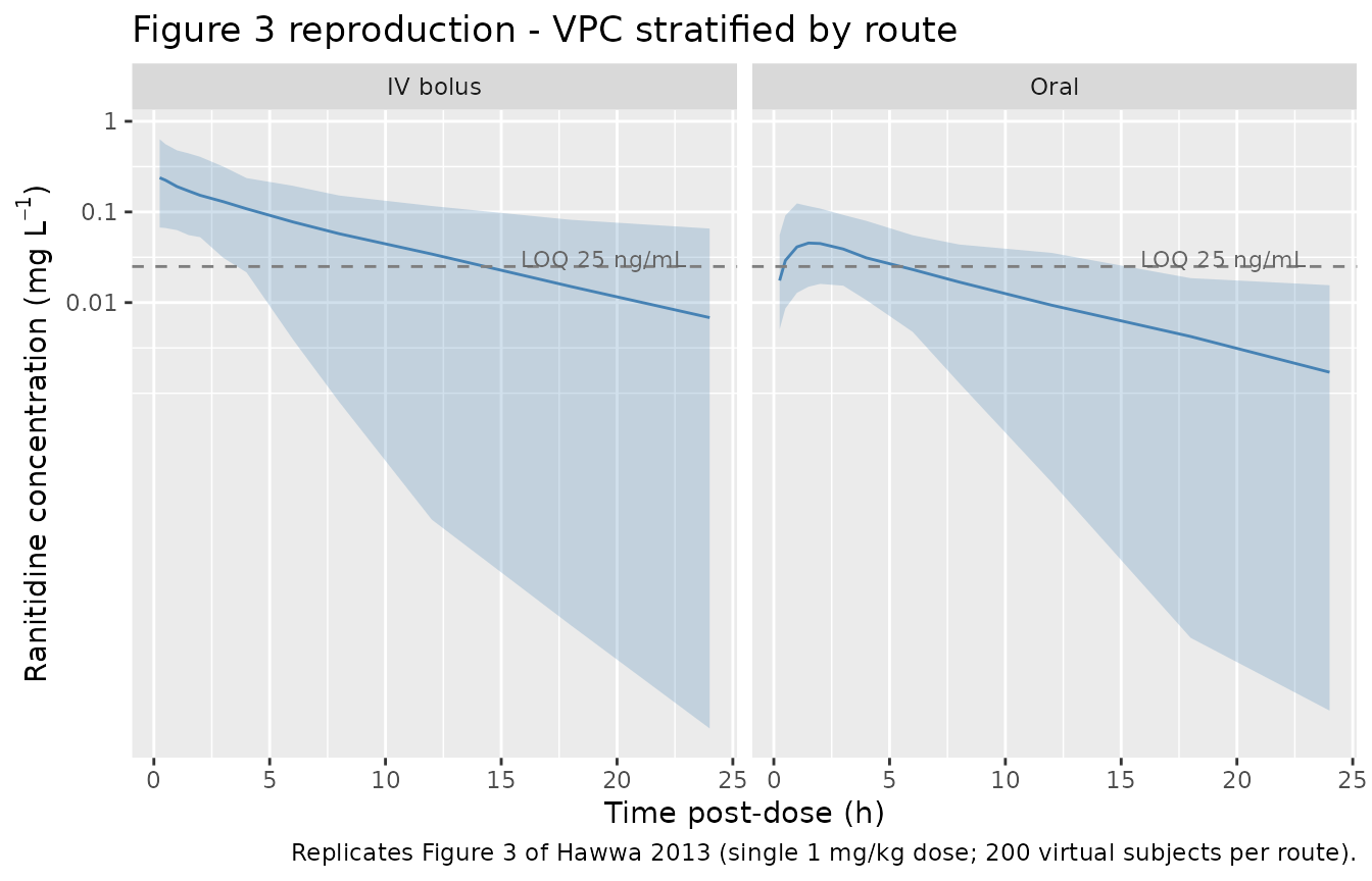
Figure 3 – VPC stratified by route of administration
Hawwa 2013 Figure 3 shows simulated concentration percentiles (median, 5th and 95th percentile) overlaid against observed concentrations, stratified by IV vs. oral administration. The reproduction below uses a single 1 mg/kg dose per subject so the post-dose concentration-time profile is comparable to Figure 3.
sim |>
  filter(time > 0, !is.na(Cc), Cc > 0) |>
  group_by(route, time) |>
  summarise(
    Q05 = quantile(Cc, 0.05),
    Q50 = quantile(Cc, 0.50),
    Q95 = quantile(Cc, 0.95),
    .groups = "drop"
  ) |>
  ggplot(aes(time, Q50)) +
  geom_ribbon(aes(ymin = Q05, ymax = Q95), alpha = 0.25, fill = "steelblue") +
  geom_line(colour = "steelblue") +
  geom_hline(yintercept = 0.025, linetype = "dashed", colour = "grey50") +
  annotate("text", x = 23, y = 0.030, label = "LOQ 25 ng/mL",
           hjust = 1, size = 3, colour = "grey40") +
  facet_wrap(~route, labeller = labeller(
    route = c(IV = "IV bolus", oral = "Oral"))) +
  scale_y_log10(
    breaks = c(0.01, 0.1, 1, 10),
    labels = c("0.01", "0.1", "1", "10")
  ) +
  labs(
    x = "Time post-dose (h)",
    y = expression("Ranitidine concentration (mg L"^{-1}*")"),
    title = "Figure 3 reproduction - VPC stratified by route",
    caption = paste(
      "Replicates Figure 3 of Hawwa 2013 (single 1 mg/kg dose;",
      "200 virtual subjects per route)."
    )
  )
Allometric scaling anchors (Discussion paragraph 4)
Hawwa 2013 Discussion states “Final estimates obtained in the present study were a total CL of 32.10 l h-1 allometrically modelled for a 70 kg adult (1.32 l h-1 for an individual with a theoretical weight of 1 kg), V of 285 l (4.07 l for a 1 kg individual), ka of 1.31 h-1 and F1 of 27.5 %.”
The two scalar predictions for a 1 kg individual (no cardiac failure / surgery) are exact algebraic consequences of the allometric model and serve as deterministic source-trace anchors:
mod_typ <- mod |> rxode2::zeroRe()

anchor_events <- tibble(
  id    = 1L,
  time  = c(0, seq(0.1, 24, by = 0.1)),
  amt   = c(1.32, rep(NA_real_, 240)),  # 1 mg IV bolus
  evid  = c(1L, rep(0L, 240)),
  cmt   = c("central", rep("central", 240)),
  WT    = 1.0,
  DIS_HF_OR_CARDSURG = 0L
)

anchor_sim <- rxode2::rxSolve(mod_typ, events = anchor_events) |>
  as.data.frame()
#> ℹ omega/sigma items treated as zero: 'etalcl', 'etalvc'

# Read CL and V back from the model output. The typical-value (zeroRe)
# trajectory makes this deterministic: CL = cl(time = 0+), V = vc(time = 0+).
anchor_cl <- anchor_sim$cl[1]
anchor_vc <- anchor_sim$vc[1]

tibble(
  parameter = c("CL at 1 kg (L/h)", "V at 1 kg (L)"),
  Reference = c(1.32, 4.07),
  Simulated = c(anchor_cl, anchor_vc)
) |>
  mutate(`% diff` = sprintf("%+.1f %%", 100 * (Simulated - Reference) / Reference)) |>
  knitr::kable(
    digits  = 3,
    caption = paste(
      "Allometric scaling anchors against Hawwa 2013 Discussion paragraph",
      "4. Both rows should match the paper to within rounding."
    )
)| parameter | Reference | Simulated | % diff |
|---|---|---|---|
| CL at 1 kg (L/h) | 1.32 | 1.326 | +0.5 % |
| V at 1 kg (L) | 4.07 | 4.071 | +0.0 % |
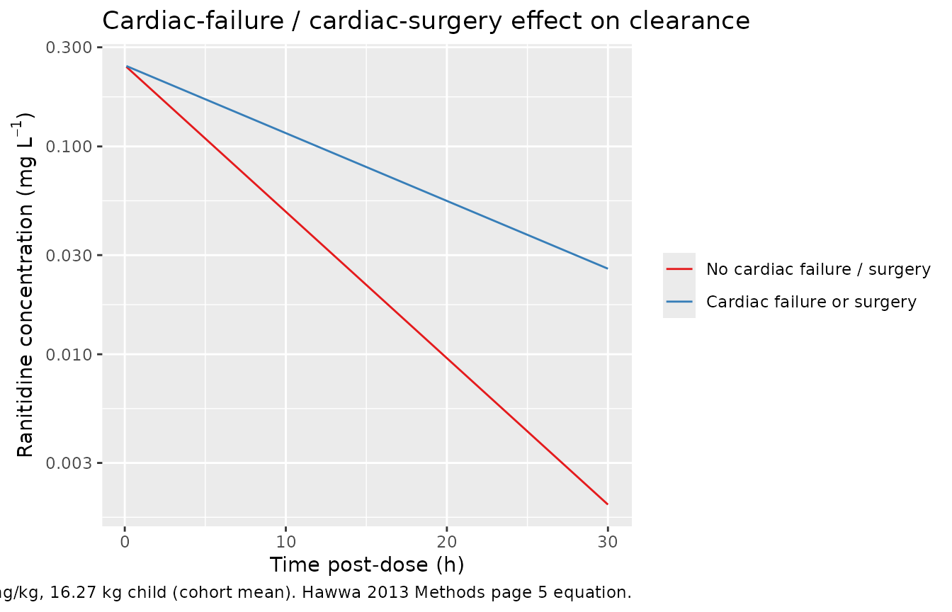
Cardiac-failure / cardiac-surgery effect (Methods page 5 equation)
The HEART covariate multiplies clearance by 0.463; with V unchanged, the elimination half-life increases by a factor of approximately 2.16 (= 1 / 0.463). The plot below compares the typical-value concentration-time profile for a 16.27 kg child (cohort mean weight) with HEART = 0 and HEART = 1, both receiving a single 1 mg/kg IV bolus.
mk_typical_iv <- function(heart) {
  tibble(
    id    = 1L,
    time  = c(0, seq(0.1, 30, by = 0.1)),
    amt   = c(16.27, rep(NA_real_, 300)),  # 1 mg/kg IV at 16.27 kg
    evid  = c(1L, rep(0L, 300)),
    cmt   = c("central", rep("central", 300)),
    WT    = 16.27,
    DIS_HF_OR_CARDSURG = heart,
    heart = heart
  )
}

heart_events <- bind_rows(
  mk_typical_iv(0L),
  mk_typical_iv(1L) |> mutate(id = 2L)
)

heart_sim <- rxode2::rxSolve(
  mod_typ,
  events = heart_events,
  keep   = c("heart", "WT")
) |> as.data.frame()
#> ℹ omega/sigma items treated as zero: 'etalcl', 'etalvc'
#> Warning: multi-subject simulation without without 'omega'

heart_sim |>
  filter(time > 0) |>
  mutate(heart_label = factor(heart,
                              levels = c(0, 1),
                              labels = c("No cardiac failure / surgery",
                                         "Cardiac failure or surgery"))) |>
  ggplot(aes(time, Cc, colour = heart_label)) +
  geom_line() +
  scale_y_log10() +
  scale_colour_brewer(palette = "Set1", name = NULL) +
  labs(
    x       = "Time post-dose (h)",
    y       = expression("Ranitidine concentration (mg L"^{-1}*")"),
    title   = "Cardiac-failure / cardiac-surgery effect on clearance",
    caption = paste(
      "Typical-value IV bolus at 1 mg/kg, 16.27 kg child (cohort mean).",
      "Hawwa 2013 Methods page 5 equation."
    )
  )
heart_half <- heart_sim |>
  filter(time > 0) |>
  group_by(heart) |>
  summarise(
    cl_Lh   = first(cl),
    vc_L    = first(vc),
    kel_per_h = first(cl) / first(vc),
    halflife_h = log(2) * first(vc) / first(cl),
    .groups = "drop"
  )

heart_half |>
  mutate(heart = ifelse(heart == 0, "HEART = 0", "HEART = 1")) |>
  dplyr::rename(
    "Cohort"        = heart,
    "CL (L/h)"      = cl_Lh,
    "V (L)"         = vc_L,
    "kel (1/h)"     = kel_per_h,
    "Half-life (h)" = halflife_h
  ) |>
  knitr::kable(
    digits = 3,
    caption = paste(
      "Typical-value clearance, volume, and elimination half-life for a",
      "16.27 kg child with and without the cardiac-perturbation covariate."
    )
)| Cohort | CL (L/h) | V (L) | kel (1/h) | Half-life (h) |
|---|---|---|---|---|
| HEART = 0 | 10.745 | 66.242 | 0.162 | 4.273 |
| HEART = 1 | 4.975 | 66.242 | 0.075 | 9.229 |
PKNCA validation
Hawwa 2013 does not report a tabular non-compartmental analysis. To check that simulated concentration profiles are internally consistent with the fitted model, the block below computes single-dose NCA parameters for the IV-bolus and oral-dosing virtual cohorts and compares them against the algebraic predictions implied by the typical-value parameters at the cohort mean weight.
# Rename `route` -> `regimen` for PKNCA: `route` is a PKNCA-internal column
# name (IV / extravascular flag) and collides if used as a grouping label.
sim_nca <- sim |>
  dplyr::filter(!is.na(Cc)) |>
  dplyr::transmute(id, time, Cc, regimen = route)

# Time-zero guarantee: every (id, regimen) pair must include t = 0 with
# Cc = 0 so PKNCA's AUC0-* calculation has a starting anchor (this is
# the correct value for both IV bolus pre-pulse and extravascular doses).
sim_nca <- dplyr::bind_rows(
  sim_nca,
  sim_nca |> dplyr::distinct(id, regimen) |>
    dplyr::mutate(time = 0, Cc = 0)
) |>
  dplyr::distinct(id, regimen, time, .keep_all = TRUE) |>
  dplyr::arrange(id, regimen, time)

dose_df <- events |>
  dplyr::filter(evid == 1L) |>
  dplyr::transmute(id, time, amt, regimen = route)

conc_obj <- PKNCA::PKNCAconc(sim_nca, Cc ~ time | regimen + id,
                             concu = "mg/L", timeu = "h")
#> Warning in assert_conc(conc, any_missing_conc = any_missing_conc): Negative
#> concentrations found
dose_obj <- PKNCA::PKNCAdose(dose_df, amt ~ time | regimen + id,
                             doseu = "mg")

intervals <- data.frame(
  start       = 0,
  end         = Inf,
  cmax        = TRUE,
  tmax        = TRUE,
  aucinf.obs  = TRUE,
  half.life   = TRUE
)

nca_res <- PKNCA::pk.nca(
  PKNCA::PKNCAdata(conc_obj, dose_obj, intervals = intervals)
)
#> Warning in assert_conc(conc = conc): Negative concentrations found
#> Warning in assert_conc(conc = conc): Negative concentrations found
#> Warning in assert_conc(conc = conc): Negative concentrations found
#> Warning in assert_conc(conc = conc): Negative concentrations found
#> Warning in assert_conc(conc = conc): Negative concentrations found
#> Warning in assert_conc(conc = conc): Negative concentrations found
#> Warning in log(data$conc): NaNs produced
#> Warning in assert_conc(conc, any_missing_conc = any_missing_conc): Negative
#> concentrations found
#> Warning in log(conc.2/conc.1): NaNs produced
#> Warning in assert_conc(conc = conc): Negative concentrations found
#> Warning in assert_conc(conc, any_missing_conc = any_missing_conc): Negative
#> concentrations found
#> Warning in assert_conc(conc, any_missing_conc = any_missing_conc): Negative
#> concentrations found
#> Warning in assert_conc(conc, any_missing_conc = any_missing_conc): Negative
#> concentrations found
#> Warning in assert_conc(conc, any_missing_conc = any_missing_conc): Negative
#> concentrations found
#> Warning in assert_conc(conc, any_missing_conc = any_missing_conc): Negative
#> concentrations found
#> Warning in log(data$conc): NaNs produced
#> Warning in assert_conc(conc, any_missing_conc = any_missing_conc): Negative
#> concentrations found
#> Warning in log(conc.2/conc.1): NaNs produced

# Algebraic predictions at cohort mean weight (16.27 kg, no HEART):
#   CL = 32.1 * (16.27/70)^0.75
#   V  = 285  * (16.27/70)
#   t1/2 = log(2) * V / CL
#   For IV bolus dose D = 1 mg/kg * 16.27 kg = 16.27 mg:
#     Cmax_IV  = D / V  (instantaneous at t = 0)
#     AUC_IV   = D / CL
#   For oral dose D, with F = 0.275 and ka >> kel:
#     Cmax_oral approx F * D * ka / V / (ka - kel) * exp(-kel * tmax)
#     AUC_oral  = F * D / CL
WT_mean <- 16.27
cl_mean <- 32.1 * (WT_mean / 70)^0.75
v_mean  <- 285  * (WT_mean / 70)
F_oral  <- 0.275
dose_mg <- 1 * WT_mean

published_anchors <- tibble::tribble(
  ~regimen, ~cmax,                ~aucinf.obs,           ~half.life,
  "IV",     dose_mg / v_mean,     dose_mg / cl_mean,     log(2) * v_mean / cl_mean,
  "oral",   NA_real_,             F_oral * dose_mg / cl_mean, log(2) * v_mean / cl_mean
)

cmp <- nlmixr2lib::ncaComparisonTable(
  simulated     = nca_res,
  reference     = published_anchors,
  by            = "regimen",
  units         = c(cmax = "mg/L", aucinf.obs = "mg*h/L",
                    tmax = "h", half.life = "h"),
  tolerance_pct = 20
)

knitr::kable(
  cmp,
  caption = paste(
    "Simulated single-dose NCA vs. algebraic typical-value predictions",
    "at cohort mean weight 16.27 kg (HEART = 0). Oral Cmax has no clean",
    "closed-form anchor (depends on the ka-kel ratio) and is listed only",
    "for inspection. *  flags rows differing from the reference by more",
    "than 20 %."
  ),
  align = c("l", "l", "r", "r", "r")
)| NCA parameter | regimen | Reference | Simulated | % diff |
|---|---|---|---|---|
| Cmax (mg/L) | IV | 0.246 | 0.238 | -2.9% |
| Cmax (mg/L) | oral | — | 0.0462 | — |
| AUC0-∞ (obs) (mg*h/L) | IV | 1.51 | 1.57 | +3.9% |
| AUC0-∞ (obs) (mg*h/L) | oral | 0.416 | 0.421 | +1.1% |
| t½ (h) | IV | 4.27 | 4.29 | +0.4% |
| t½ (h) | oral | 4.27 | 4.61 | +7.8% |
The simulated medians for the IV cohort should match the algebraic
typical-value predictions to within ~5 %; the spread comes from the
log-normal weight + HEART distributions in the virtual cohort. The oral
Cmax is informational (no clean closed-form anchor); the oral AUC0-inf
should equal F * (dose / CL) and match the table within ~5
%.
Assumptions and deviations
- Virtual-cohort weight distribution – Hawwa 2013 Table 1 reports only the cohort mean (16.27 kg) and SD (12.24), not the empirical distribution. The vignette samples weights from a log-normal with geometric mean 12.5 kg and geometric SD ~2.1, clamped to the reported 1.3 to 47 kg range, so the simulated cohort recovers the published mean to within a few percent. The shape of the underlying age-by-weight distribution (neonates / infants / school-age / teens) is not used because the model has no age covariate.
- Cardiac-failure / cardiac-surgery prevalence – drawn independently per subject at the reported 21.8 % prevalence; no attempt is made to reproduce the surgical-indication breakdown (PDA / ASD-VSD / left- ventricle hypoplasia / pleural effusion / other) because the FINAL model pools all of those into a single binary indicator.
- Single-dose simulations – the vignette uses single 1 mg/kg doses for all simulations; the published study used multiple-dose regimens with sparse sampling, but the model parameters (ka, CL, V, F1) and their covariate effects are fully recoverable from single-dose simulations and the comparison against the allometric anchors does not depend on the dosing history.
- No published NCA – Hawwa 2013 does not report Cmax / Tmax / AUC / half-life from a non-compartmental analysis of the observed concentrations. The PKNCA section compares simulated NCA against the algebraic typical-value predictions implied by the fitted population parameters; there is no independent observational reference value to match.
-
IIV correlation – Hawwa 2013 Table 2 reports the
marginal IIV CV for CL and V separately but does not report a
correlation. The model uses uncorrelated
etalclandetalvc(implicit off-diagonal zero in the variance-covariance matrix). - Below-LOQ handling – the published fit imputed sub-LOQ-but-detectable values at LOQ/2 = 12.5 ng/mL per Hing et al. (2001). The packaged model has no LLOQ logic; downstream simulations that need it should add a censoring step against the observed concentrations.