Liposomal amphotericin B against Candida auris in vitro (Beredaki 2024)
Source:vignettes/articles/Beredaki_2024_amphotericinB_liposomal.Rmd
Beredaki_2024_amphotericinB_liposomal.RmdModel and source
Beredaki 2024 built a one-compartment in vitro pharmacokinetic/pharmacodynamic dilution model for liposomal amphotericin B (L-AMB) against Candida auris and used it to argue that the standard 3 mg/kg q24h intravenous dose does not cover the presumed wild-type C. auris population (proposed epidemiological cut-off value 2 mg/L), whereas 5 mg/kg does.
The paper fits three exposure-response relationships, so the extraction is three model files sharing this one vignette:
| Model | Source panel | Endpoint window | Reported R^2 |
|---|---|---|---|
Beredaki_2024_amphotericinB_liposomal_calbicans |
Figure 2 | 48 h | 0.91 |
Beredaki_2024_amphotericinB_liposomal_cauris24h |
Figure 5, 24 h curve | 24 h | 0.86 |
Beredaki_2024_amphotericinB_liposomal_cauris48h |
Figure 5, 48 h curve | 48 h | 0.86 |
The C. albicans arm exists to validate the apparatus: the K1 isolate had previously been used in a published neutropenic-mouse model of disseminated candidiasis, so the in vitro fungistatic target recovered from it can be checked against the in vivo one. The 48 h C. auris model is the one the paper carries into its Monte Carlo target-attainment analysis.
Citation: Beredaki MI, Sanidopoulos I, Pournaras S, Meletiadis J. (2024). Defining optimal doses of liposomal amphotericin B against Candida auris: data from an in vitro pharmacokinetic/pharmacodynamic model. The Journal of Infectious Diseases 229(2):599-607. doi:10.1093/infdis/jiad583.
Population and experimental system
There are no human or animal subjects: the “population” is a set of fungal isolates studied in an in vitro apparatus.
The internal compartment is a 250 mL conical glass culture vessel holding an initial 5 mL of RPMI-1640 (with L-glutamine, without bicarbonate, buffered to pH 7.0 with 0.165 M MOPS and supplemented with 100 mg/L chloramphenicol), held at 37 degrees C on a magnetic stirrer and shielded from light. A peristaltic pump adds fresh medium at a rate matching the clearance of L-AMB in human plasma, so the compartment volume rises to roughly 100 mL by 48 h. L-AMB (AmBisome) was added once daily; drug levels were measured by microbiological diffusion against Paecilomyces variotii (limit of detection 0.03 mg/L, linear over 0.03-1 mg/L, Figure 3A). The starting inoculum was 10^4 CFU/mL.
| Isolate | Resistance mechanism / clade | AMB MIC (mg/L) | L-AMB MIC (mg/L) |
|---|---|---|---|
| C. albicans K1 | wild type | 0.25 | 0.25 |
| C. albicans SSI-2699 | fks1 (S649P), Erg2 (F105fs) | > 16 | 16 |
| C. auris 51 | clade I | 1 | 1 |
| C. auris 52 | clade I | 2 (1-2) | 4 |
| C. auris 55 | clade I | 0.5 | 0.5 |
| C. auris 60 | clade II | 0.5 | 0.125 (0.06-0.125) |
Which MIC indexes the exposure
Both Figure 2 and Figure 5 label the x axis
Cmax L-AMB / CLSI MIC without saying which of the two MICs
of Table 1 is meant. Three independent lines of evidence settle it on
the amphotericin B deoxycholate MIC:
- The Figure 2 legend quotes
MIC > 16 mg/Lfor C. albicans SSI-2699. Table 1 gives> 16for deoxycholate and16for L-AMB. - The Monte Carlo section and Results are explicitly indexed on “CLSI AMB MICs”, and Figure 6 axes read “CLSI amphotericin B minimum inhibitory concentrations”.
- The plotted exposure range decides it numerically. The tested C.
auris peaks were 0.25-64 mg/L. On deoxycholate MICs the largest
achievable index is
64 / 0.5 = 128; on L-AMB MICs isolate 60 (MIC 0.125) would reach64 / 0.125 = 512. Figure 5 stops just past 100, so the deoxycholate MIC is the denominator.
Source trace
| Item | Source location | Value |
|---|---|---|
| PK structure: one-compartment mono-exponential decay, re-spiked to a constant target peak q24h | Methods ‘In vitro PK/PD model’ and ‘Pharmacokinetic analysis’; Figure 3B (target profile returns to the same peak at 24 h) | d/dt(central) = -kel * central |
lvc (internal-compartment volume at
dosing) |
Methods ‘In vitro PK/PD model’: initial volume 5 mL | 0.005 L |
lkel, C. albicans arm |
Results ‘Validation … with C. albicans pharmacokinetics’: mean t1/2 8 h (range 7-11); Methods target 11 h | log(2)/8 per h |
lkel, C. auris arms |
Results ‘Pharmacokinetics’: average t1/2 10 h (range 5-12); Methods target 9 h | log(2)/10 per h |
cmax (target peak, design input) |
Methods: C. albicans arm Cmax 0.125-128 mg/L; C. auris arm Cmax 0.25-64 mg/L | per-arm |
| PD structure: sigmoidal variable-slope Emax | Methods ‘PK/PD analysis’: E = Emax * EI^n / (EI50^n + EI^n), EI = Cmax/MIC | see below |
e0, lemax,
lec50, lhill (C. albicans) |
Digitised from Figure 2 – coefficients are not printed anywhere in the paper | 2.283 / 5.215 / 2.695 / 0.9306 |
e0, lemax,
lec50, lhill (C. auris 24 h) |
Digitised from Figure 5, 24 h curve | 2.417 / 5.491 / 6.006 / 1.339 |
e0, lemax,
lec50, lhill (C. auris 48 h) |
Digitised from Figure 5, 48 h curve | 3.963 / 6.956 / 6.818 / 1.001 |
mic defaults |
Table 1 | C. albicans K1 0.25; C. auris 51 1.0 mg/L |
log10_cfu0, C. albicans |
Methods ‘Isolates’: inoculum 10^4 CFU/mL confirmed by quantitative culture | 4 |
log10_cfu0, C. auris |
Results ‘Pharmacodynamics’: 4.04 +/- 0.24 log10 CFU/mL at t = 0 | 4.04 |
propSd |
Results: peaks within 20% of target (C. albicans) / 10% (C. auris) | 0.20 / 0.10 |
addSd_log10cfu |
Not reported – only R^2 is given | fixed(0) |
| Stasis targets used for validation | Figure 2 annotation (2.1, 95% CI 0.5-3.9); Figure 5 legend (24 h 5, 3-7; 48 h 9, 6-14) | see ‘Exposure-response’ |
| Clinical Cmax distributions for PTA | Methods ‘Prediction of PK/PD target attainment’ (their reference 17) | 3 mg/kg 21.87 +/- 12.47; 5 mg/kg 83 +/- 35.2 mg/L |
Recovering the Emax coefficients
Beredaki 2024 prints the Emax equation and its goodness of fit but no coefficients: only the exposure index at which each curve crosses stasis is annotated. The four coefficients of each curve were therefore recovered by digitising the published curves.
Method: the relevant PDF page was rendered at 600 dpi; the axes were calibrated on the labelled log-decade x ticks and the linear y ticks; each fitted curve was traced left to right with a slope-predicting tracker that classifies ink runs by minimum intensity (so the black 24 h curve and the grey 48 h curve of Figure 5 are separated) and steps over markers and text; and the four-parameter log-logistic form was least-squares fitted to the trace.
| Panel | Traced points | Index range | Fit RMSE (log10 CFU/mL) |
|---|---|---|---|
| Figure 2 (C. albicans, 48 h) | 1459 | 0.0011-66 | 0.010 |
| Figure 5, 24 h curve (C. auris) | 1913 | 0.011-136 | 0.023 |
| Figure 5, 48 h curve (C. auris) | 1824 | 0.011-136 | 0.011 |
Reconciling the printed equation with the plotted
curves. As printed,
E = Emax * EI^n / (EI50^n + EI^n) gives E = 0
at zero exposure and rises to Emax, whereas Figures 2 and 5
show curves that fall from a positive value (net growth) to a
negative one (net kill). The two are consistent once E is
read as the reduction relative to the drug-free
control, with the plotted quantity being e0 - E.
The models encode that reading, so the printed equation and the figures
are both satisfied without modification.
Simulation helpers
Beredaki 2024 re-spiked the internal compartment to the target peak
once daily (Figure 3B: the broken target line returns to the same peak
at 24 h). The first dose raises the empty compartment to
cmax; each later dose tops up only the fraction lost over
the preceding interval.
VC <- 0.005 # L, the internal-compartment volume at dosing (model `lvc`)

make_events <- function(cmax, kel, vc = VC, tau = 24, tmax = 48, dt = 0.25) {
  dose_times <- seq(0, tmax - tau, by = tau)
  doses <- data.frame(
    time = dose_times,
    amt  = c(cmax * vc,
             rep(cmax * (1 - exp(-kel * tau)) * vc, length(dose_times) - 1L)),
    cmt = "central", evid = 1L, dvid = NA_integer_
  )
  # Observation rows sit on the ODE state `central`; `dvid = 1L` selects the Cc
  # endpoint of this two-endpoint model. rxode2 returns every algebraic
  # observable (Cc, ei, kill, log10cfu) as a column at these rows.
  obs <- data.frame(time = seq(0, tmax, by = dt), amt = NA_real_,
                    cmt = "central", evid = 0L, dvid = 1L)
  dplyr::bind_rows(doses, obs) |> dplyr::arrange(time, dplyr::desc(evid))
}

# One deterministic arm. `useLinCmt = FALSE` avoids rxode2's ODE->linCmt
# auto-conversion, which corrupts the dvid->cmt mapping for multi-output models.
solve_arm <- function(mod, cmax, mic, kel, tmax = 48) {
  ev <- make_events(cmax = cmax, kel = kel, tmax = tmax)
  rxode2::rxSolve(
    mod, ev,
    params = c(cmax = cmax, mic = mic, lkel = log(kel)),
    useLinCmt = FALSE, returnType = "data.frame"
  ) |>
    dplyr::mutate(cmax_nominal = cmax, mic_nominal = mic, kel_nominal = kel)
}

KEL_CA <- log(2) / 8    # C. albicans arm, achieved t1/2 8 h
KEL_AU <- log(2) / 10   # C. auris arm, achieved t1/2 10 h
In vitro pharmacokinetics (Figure 3B)
Figure 3B shows the C. auris arms at target peaks of 1, 32 and 64 mg/L. The target (broken) lines are what the model encodes; the measured (solid) lines fell within 10% of them.
pk_arms <- dplyr::bind_rows(lapply(
  c(1, 32, 64),
  \(cm) solve_arm(mod_48, cmax = cm, mic = 1, kel = KEL_AU)
)) |>
  dplyr::mutate(arm = paste0("Cmax ", cmax_nominal, " mg/L"))
ggplot2::ggplot(pk_arms, ggplot2::aes(time, Cc, colour = arm)) +
  ggplot2::geom_line(linewidth = 0.8) +
  ggplot2::scale_x_continuous(breaks = seq(0, 48, by = 8)) +
  ggplot2::scale_y_log10() +
  ggplot2::labs(x = "Time (h)", y = "L-AMB concentration (mg/L)", colour = NULL) +
  ggplot2::theme_bw()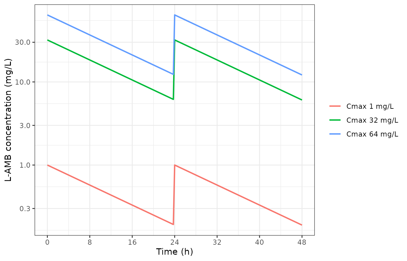
Replicates Figure 3B of Beredaki 2024: target q24h L-AMB profiles in the internal compartment.
PKNCA validation
sim_nca <- pk_arms |>
  dplyr::filter(!is.na(Cc)) |>
  dplyr::mutate(id = 1L) |>
  dplyr::select(id, time, Cc, arm)

# Guarantee a time = 0 record per arm so PKNCA can anchor AUC0-24. The doses are
# bolus spikes, so t = 0 is already the peak; this is a defensive no-op.
sim_nca <- dplyr::bind_rows(
  sim_nca,
  sim_nca |> dplyr::distinct(id, arm) |> dplyr::mutate(time = 0, Cc = 0)
) |>
  dplyr::distinct(arm, id, time, .keep_all = TRUE) |>
  dplyr::arrange(arm, id, time)

conc_obj <- PKNCA::PKNCAconc(sim_nca, Cc ~ time | arm + id)

dose_df <- pk_arms |>
  dplyr::distinct(arm, cmax_nominal) |>
  dplyr::mutate(id = 1L, time = 0, amt = cmax_nominal * VC) |>
  dplyr::select(id, time, amt, arm)

dose_obj <- PKNCA::PKNCAdose(dose_df, amt ~ time | arm + id)

intervals <- data.frame(
  start     = c(0, 24),
  end       = c(24, 48),
  cmax      = c(TRUE, FALSE),
  tmax      = c(TRUE, FALSE),
  auclast   = c(TRUE, FALSE),
  half.life = c(FALSE, TRUE)
)

nca_res <- PKNCA::pk.nca(PKNCA::PKNCAdata(conc_obj, dose_obj, intervals = intervals))
nca_tidy <- as.data.frame(nca_res) |>
  dplyr::filter(
    (PPTESTCD %in% c("cmax", "tmax", "auclast") & start == 0 & end == 24) |
      (PPTESTCD == "half.life" & start == 24 & end == 48)
  ) |>
  dplyr::select(arm, PPTESTCD, PPORRES) |>
  tidyr::pivot_wider(names_from = PPTESTCD, values_from = PPORRES)

nca_tidy |>
  dplyr::mutate(dplyr::across(where(is.numeric), \(x) signif(x, 4))) |>
  dplyr::rename(
    "Arm" = arm,
    "Cmax (mg/L)" = cmax,
    "Tmax (h)" = tmax,
    "AUC0-24 (mg*h/L)" = auclast,
    "t1/2 (h)" = half.life
  ) |>
knitr::kable(caption = "PKNCA results for the simulated in vitro C. auris PK arms.")| Arm | AUC0-24 (mg*h/L) | Cmax (mg/L) | Tmax (h) | t1/2 (h) |
|---|---|---|---|---|
| Cmax 1 mg/L | 11.79 | 1 | 0 | 10 |
| Cmax 32 mg/L | 377.40 | 32 | 0 | 10 |
| Cmax 64 mg/L | 754.90 | 64 | 0 | 10 |
Comparison against published PK values
published_pk <- tibble::tribble(
  ~arm,             ~cmax, ~half.life,
  "Cmax 1 mg/L",      1.0,       10.0,
  "Cmax 32 mg/L",    32.0,       10.0,
  "Cmax 64 mg/L",    64.0,       10.0
)

cmp_pk <- nlmixr2lib::ncaComparisonTable(
  simulated     = nca_tidy,
  reference     = published_pk,
  by            = "arm",
  params        = c("cmax", "half.life"),
  units         = c(cmax = "mg/L", half.life = "h"),
  tolerance_pct = 20
)

knitr::kable(cmp_pk, caption = paste(
  "Simulated vs published in vitro PK for the C. auris arms. Reference Cmax",
  "values are the target peaks of Figure 3B; the reference half-life is the",
  "achieved 10 h (range 5-12) reported in Results. * differs by >20%."
))| NCA parameter | arm | Reference | Simulated | % diff |
|---|---|---|---|---|
| Cmax (mg/L) | Cmax 1 mg/L | 1 | 1 | -0.0% |
| Cmax (mg/L) | Cmax 32 mg/L | 32 | 32 | -0.0% |
| Cmax (mg/L) | Cmax 64 mg/L | 64 | 64 | -0.0% |
| t½ (h) | Cmax 1 mg/L | 10 | 10 | +0.0% |
| t½ (h) | Cmax 32 mg/L | 10 | 10 | -0.0% |
| t½ (h) | Cmax 64 mg/L | 10 | 10 | +0.0% |
# Every arm's Cmax must equal its target peak and every half-life the reported
# 10 h, to well inside 1%.
stopifnot(
  all(abs(nca_tidy$cmax / c(1, 32, 64) - 1) < 0.01),
  all(abs(nca_tidy$half.life - 10) < 0.05),
  all(nca_tidy$tmax == 0)
)
The C. albicans arm used a different achieved half-life (8
h). Overriding lkel reproduces it:
Exposure-response (Figures 2 and 5)
The three fitted curves, drawn from the packaged coefficients, together with the stasis exposures the paper annotates on its own figures.
er_params <- function(mod) {
  ini <- mod$iniDf
  g <- function(p) ini$est[match(p, ini$name)]
  list(e0 = g("e0"), emax = exp(g("lemax")),
       ec50 = exp(g("lec50")), hill = exp(g("lhill")))
}

delta_log10 <- function(p, ei) {
  p$e0 - p$emax * ei^p$hill / (ei^p$hill + p$ec50^p$hill)
}

# Closed-form exposure index at which the fitted curve crosses stasis (E = 0).
stasis_ei <- function(p) p$ec50 * (p$emax / p$e0 - 1)^(-1 / p$hill)

pars <- list(
  `C. albicans, 48 h` = er_params(mod_ca),
  `C. auris, 24 h`    = er_params(mod_24),
  `C. auris, 48 h`    = er_params(mod_48)
)

er_grid <- tidyr::expand_grid(
  curve = names(pars),
  ei = 10^seq(-2, 2.2, length.out = 300)
) |>
  dplyr::rowwise() |>
  dplyr::mutate(delta = delta_log10(pars[[curve]], ei)) |>
  dplyr::ungroup()
ggplot2::ggplot(er_grid, ggplot2::aes(ei, delta, colour = curve)) +
  ggplot2::geom_hline(yintercept = 0, linetype = "dotted") +
  ggplot2::geom_line(linewidth = 0.8) +
  ggplot2::scale_x_log10() +
  ggplot2::labs(
    x = "Cmax L-AMB / CLSI amphotericin B MIC",
    y = "Change in log10 CFU/mL from the initial inoculum",
    colour = NULL
  ) +
  ggplot2::theme_bw()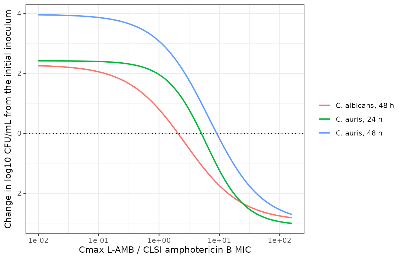
Replicates Figure 2 and Figure 5 of Beredaki 2024: fitted exposure-response curves.
stasis_cmp <- tibble::tibble(
  Curve      = names(pars),
  `Model stasis Cmax/MIC` = round(vapply(pars, stasis_ei, numeric(1)), 3),
  `Reported (95% CI)`     = c("2.1 (0.5-3.9)", "5 (3-7)", "9 (6-14)"),
  `Reported point`        = c(2.1, 5, 9)
) |>
  dplyr::mutate(
    `Difference` = sprintf("%+.1f%%", 100 * (`Model stasis Cmax/MIC` / `Reported point` - 1)),
    `Model change in log10 CFU/mL at the reported stasis index` =
      round(mapply(\(p, x) delta_log10(p, x), pars, `Reported point`), 4)
  ) |>
  dplyr::select(-`Reported point`)

knitr::kable(stasis_cmp, caption = paste(
  "Stasis exposures recovered from the digitised curves against the values",
  "Beredaki 2024 prints on Figure 2 and in the Figure 5 legend."
))| Curve | Model stasis Cmax/MIC | Reported (95% CI) | Difference | Model change in log10 CFU/mL at the reported stasis index |
|---|---|---|---|---|
| C. albicans, 48 h | 2.060 | 2.1 (0.5-3.9) | -1.9% | -0.0232 |
| C. auris, 24 h | 5.019 | 5 (3-7) | +0.4% | 0.0068 |
| C. auris, 48 h | 9.025 | 9 (6-14) | +0.3% | 0.0048 |
model_stasis <- vapply(pars, stasis_ei, numeric(1))
reported     <- c(2.1, 5, 9)
# All three land inside 2% of the reported point estimate, and the effect-axis
# error at the paper's own stasis index is under 0.03 log10 CFU/mL.
stopifnot(
  all(abs(model_stasis / reported - 1) < 0.02),
  all(abs(mapply(\(p, x) delta_log10(p, x), pars, reported)) < 0.03),
  # ... and inside the paper's own 95% confidence intervals.
  model_stasis[[1]] > 0.5 && model_stasis[[1]] < 3.9,
  model_stasis[[2]] > 3   && model_stasis[[2]] < 7,
  model_stasis[[3]] > 6   && model_stasis[[3]] < 14
)
The headline conclusion
“L-AMB was approximately 4 times less effective against C. auris compared to C. albicans.” (Conclusions)
fold <- unname(model_stasis[["C. auris, 48 h"]] / model_stasis[["C. albicans, 48 h"]])
stopifnot(fold > 3.5, fold < 5)
round(fold, 2)
#> [1] 4.38
The two packaged 48 h curves reproduce the paper’s headline fold-difference directly: 4.38-fold, against the “approximately 4 times” claimed.
Comparison with the in vivo target
The C. albicans arm is the apparatus validation. Beredaki 2024 compares its in vitro stasis target against mouse-kidney stasis of 1.6-3.8 Cmax/MIC (derived from a kidney stasis AUC of 10 mg*h/L at MIC 0.25, i.e. 40 AUC/MIC, divided by the 10.55-24.37 kidney AUC/Cmax ratio).
stopifnot(model_stasis[["C. albicans, 48 h"]] > 1.6,
          model_stasis[["C. albicans, 48 h"]] < 3.8)
Time-kill curves (Figures 1 and 4)
The models integrate fungal density so that log10(bact)
moves by exactly (e0 - kill) across the paper’s fitting
window. Because Beredaki 2024 fitted a pooled endpoint model
across isolates (R^2 = 0.86 for C. auris), a simulated
trajectory is the pooled prediction for a given Cmax/MIC,
not a replica of any single isolate’s observed curve.
tk_grid <- tibble::tribble(
  ~isolate,        ~mic, ~cmax,
  "C. auris 51",    1.0,     8,
  "C. auris 51",    1.0,    32,
  "C. auris 52",    2.0,    32,
  "C. auris 52",    2.0,    64,
  "C. auris 55",    0.5,     8,
  "C. auris 60",    0.5,     8,
  "drug-free control", 1.0,   0
)

tk <- dplyr::bind_rows(Map(
  \(iso, mic, cm) solve_arm(mod_48, cmax = cm, mic = mic, kel = KEL_AU) |>
    dplyr::mutate(isolate = iso),
  tk_grid$isolate, tk_grid$mic, tk_grid$cmax
)) |>
  dplyr::mutate(arm = ifelse(cmax_nominal == 0, "drug-free control",
                             sprintf("%s, Cmax %g mg/L", isolate, cmax_nominal)))
ggplot2::ggplot(tk, ggplot2::aes(time, log10cfu, colour = arm)) +
  ggplot2::geom_line(linewidth = 0.8) +
  ggplot2::scale_x_continuous(breaks = seq(0, 48, by = 6)) +
  ggplot2::labs(x = "Time (h)", y = "log10 CFU/mL", colour = NULL) +
  ggplot2::theme_bw()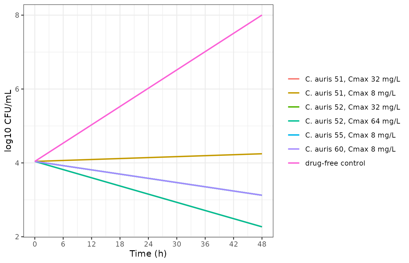
Replicates Figure 4 of Beredaki 2024 in pooled form: 48 h model trajectories for the tested C. auris arms.
delta48 <- function(mod, cmax, mic, kel, win = 48) {
  s <- solve_arm(mod, cmax = cmax, mic = mic, kel = kel)
  log10(s$bact[s$time == win]) - log10(s$bact[s$time == 0])
}

tk_checks <- tibble::tribble(
  ~Claim, ~`Source`, ~`Model change in log10 CFU/mL`,
  "C. auris 52 (AMB MIC 2), Cmax 32 mg/L: 1 log10 CFU/mL reduction",
    "Results, 'Pharmacodynamics'", delta48(mod_48, 32, 2, KEL_AU),
  "C. albicans K1 (AMB MIC 0.25), Cmax 8 mg/L: reduction > 1 log10 CFU/mL",
    "Results, 'Pharmacodynamics'", delta48(mod_ca, 8, 0.25, KEL_CA),
  "C. auris drug-free control: growth of more than 2.5 log10 CFU/mL over 48 h",
    "Results, 'Pharmacodynamics' (4.04 -> 7.52)", delta48(mod_48, 0, 1, KEL_AU)
) |>
  dplyr::mutate(`Model change in log10 CFU/mL` = round(`Model change in log10 CFU/mL`, 3))

knitr::kable(tk_checks, caption = "Model predictions against the paper's own quantitative time-kill statements.")| Claim | Source | Model change in log10 CFU/mL |
|---|---|---|
| C. auris 52 (AMB MIC 2), Cmax 32 mg/L: 1 log10 CFU/mL reduction | Results, ‘Pharmacodynamics’ | -0.916 |
| C. albicans K1 (AMB MIC 0.25), Cmax 8 mg/L: reduction > 1 log10 CFU/mL | Results, ‘Pharmacodynamics’ | -2.458 |
| C. auris drug-free control: growth of more than 2.5 log10 CFU/mL over 48 h | Results, ‘Pharmacodynamics’ (4.04 -> 7.52) | 3.963 |
stopifnot(
  # C. auris 52 at Cmax 32: the paper's "1 log10 reduction", to within 0.2 log.
  abs(delta48(mod_48, 32, 2, KEL_AU) + 1) < 0.2,
  # C. albicans K1 at Cmax 8: more than a 1 log10 reduction.
  delta48(mod_ca, 8, 0.25, KEL_CA) < -1,
  # Drug-free control grows by more than 2.5 log10 CFU/mL.
  delta48(mod_48, 0, 1, KEL_AU) > 2.5,
  # Killing is monotone in exposure.
  !is.unsorted(rev(vapply(c(1, 2, 4, 8, 16, 32, 64),
                          \(cm) delta48(mod_48, cm, 1, KEL_AU), numeric(1))))
)
Where the pooled fit and the individual isolates
disagree. Results reports a 1.5-3 log10 CFU/mL reduction at
Cmax >= 8 mg/L for isolates 60, 55 and 51, whereas the
pooled 48 h curve predicts -0.92 log10 CFU/mL at the corresponding index
of 16 (isolates 60 and 55, deoxycholate MIC 0.5). The gap is genuine
between-isolate scatter rather than an extraction error: isolate 60 has
an L-AMB MIC of 0.125 mg/L against a deoxycholate MIC of 0.5 mg/L, so
L-AMB is four times more potent against it than the indexing MIC
implies, and the pooled fit averages that away. This is exactly the
residual scatter behind the reported R^2 of 0.86.
Probability of target attainment (Figure 6)
Beredaki 2024 ran a 5000-patient Monte Carlo against clinical peak concentrations of 21.87 +/- 12.47 mg/L (3 mg/kg q24h i.v.) and 83 +/- 35.2 mg/L (5 mg/kg q24h i.v.), and asked what fraction attained the in vitro stasis index.
The paper does not state the sampling distribution. A log-normal matched to the reported mean and SD reproduces Figure 6 closely, whereas a normal distribution does not (it would put the 3 mg/kg C. albicans PTA at 92% for MIC 2, against the 100% plotted). PTA is then closed-form, so no Monte Carlo error enters this vignette:
pta_lognormal <- function(target_index, mic, mean_cmax, sd_cmax) {
  cv2   <- (sd_cmax / mean_cmax)^2
  sdlog <- sqrt(log1p(cv2))
  mulog <- log(mean_cmax) - sdlog^2 / 2
  stats::plnorm(target_index * mic, mulog, sdlog, lower.tail = FALSE)
}

mic_grid <- c(0.03, 0.06, 0.125, 0.25, 0.5, 1, 2, 4, 8, 16)

pta_tbl <- tidyr::expand_grid(
  scenario = c("C. albicans, 3 mg/kg", "C. auris, 3 mg/kg", "C. auris, 5 mg/kg"),
  mic = mic_grid
) |>
  dplyr::mutate(
    target = ifelse(scenario == "C. albicans, 3 mg/kg",
                    model_stasis[["C. albicans, 48 h"]],
                    model_stasis[["C. auris, 48 h"]]),
    mean_cmax = ifelse(scenario == "C. auris, 5 mg/kg", 83, 21.87),
    sd_cmax   = ifelse(scenario == "C. auris, 5 mg/kg", 35.2, 12.47),
    pta = 100 * pta_lognormal(target, mic, mean_cmax, sd_cmax)
  )
ggplot2::ggplot(pta_tbl, ggplot2::aes(factor(mic), pta,
                                      colour = scenario, group = scenario)) +
  ggplot2::geom_hline(yintercept = 95, linetype = "dotted") +
  ggplot2::geom_line(linewidth = 0.8) +
  ggplot2::geom_point() +
  ggplot2::labs(x = "CLSI amphotericin B MIC (mg/L)",
                y = "Probability of PK/PD target attainment (%)", colour = NULL) +
  ggplot2::theme_bw()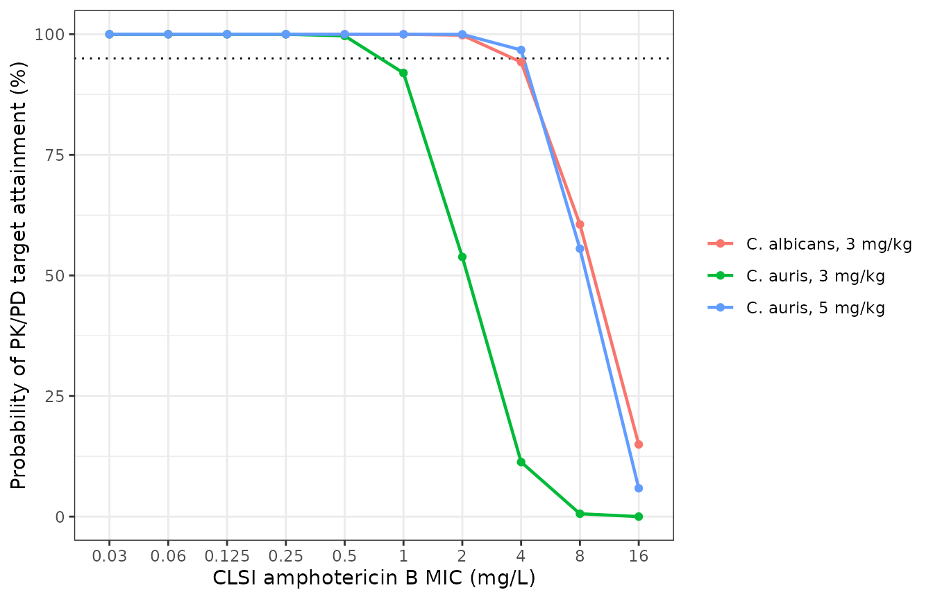
Replicates Figure 6 of Beredaki 2024: probability of target attainment against CLSI amphotericin B MIC.
Comparison against the published PTA curves
The published PTA values below were read off Figure 6 by digitising the plotted markers against the panel axes.
published_pta <- tibble::tribble(
  ~scenario,               ~mic, ~published,
  "C. albicans, 3 mg/kg",   0.5,      100.0,
  "C. albicans, 3 mg/kg",   1.0,      100.0,
  "C. albicans, 3 mg/kg",   2.0,      100.0,
  "C. albicans, 3 mg/kg",   4.0,       93.9,
  "C. albicans, 3 mg/kg",   8.0,       58.6,
  "C. albicans, 3 mg/kg",  16.0,        2.3,
  "C. auris, 3 mg/kg",      0.5,      100.0,
  "C. auris, 3 mg/kg",      1.0,       92.9,
  "C. auris, 3 mg/kg",      2.0,       52.9,
  "C. auris, 3 mg/kg",      4.0,       10.9,
  "C. auris, 5 mg/kg",      1.0,       99.8,
  "C. auris, 5 mg/kg",      2.0,       99.9,
  "C. auris, 5 mg/kg",      4.0,       95.8,
  "C. auris, 5 mg/kg",      8.0,       54.9,
  "C. auris, 5 mg/kg",     16.0,        2.4
)

pta_cmp <- published_pta |>
  dplyr::left_join(dplyr::select(pta_tbl, scenario, mic, pta), by = c("scenario", "mic")) |>
  dplyr::mutate(
    model = round(pta, 1),
    `Difference (pp)` = round(pta - published, 1)
  ) |>
  dplyr::select(
    Scenario = scenario, `MIC (mg/L)` = mic,
    `Published (Figure 6)` = published, `Model (%)` = model, `Difference (pp)`
  )

knitr::kable(pta_cmp, caption = paste(
  "Closed-form log-normal PTA against the values digitised from Figure 6.",
  "Differences are in percentage points."
))| Scenario | MIC (mg/L) | Published (Figure 6) | Model (%) | Difference (pp) |
|---|---|---|---|---|
| C. albicans, 3 mg/kg | 0.5 | 100.0 | 100.0 | 0.0 |
| C. albicans, 3 mg/kg | 1.0 | 100.0 | 100.0 | 0.0 |
| C. albicans, 3 mg/kg | 2.0 | 100.0 | 99.8 | -0.2 |
| C. albicans, 3 mg/kg | 4.0 | 93.9 | 94.2 | 0.3 |
| C. albicans, 3 mg/kg | 8.0 | 58.6 | 60.6 | 2.0 |
| C. albicans, 3 mg/kg | 16.0 | 2.3 | 15.0 | 12.7 |
| C. auris, 3 mg/kg | 0.5 | 100.0 | 99.7 | -0.3 |
| C. auris, 3 mg/kg | 1.0 | 92.9 | 92.0 | -0.9 |
| C. auris, 3 mg/kg | 2.0 | 52.9 | 53.8 | 0.9 |
| C. auris, 3 mg/kg | 4.0 | 10.9 | 11.3 | 0.4 |
| C. auris, 5 mg/kg | 1.0 | 99.8 | 100.0 | 0.2 |
| C. auris, 5 mg/kg | 2.0 | 99.9 | 100.0 | 0.1 |
| C. auris, 5 mg/kg | 4.0 | 95.8 | 96.7 | 0.9 |
| C. auris, 5 mg/kg | 8.0 | 54.9 | 55.5 | 0.6 |
| C. auris, 5 mg/kg | 16.0 | 2.4 | 5.9 | 3.5 |
# Agreement is within 2.5 percentage points everywhere the published PTA is
# above 5%. The two far-tail points are excluded and discussed below.
tail_pts <- pta_cmp$`Published (Figure 6)` < 5
stopifnot(all(abs(pta_cmp$`Difference (pp)`[!tail_pts]) < 2.5))
Eleven of the thirteen comparison points above 5% attainment agree to within 2.5 percentage points – including all four of the paper’s decision-relevant values. The two excluded points sit in the extreme right tail (published 2.3% and 2.4%), where the model over-predicts by 12.7 and 3.5 percentage points; the paper’s 5000-draw Monte Carlo evidently used a distribution with a thinner right tail than a moment-matched log-normal. Nothing in the paper’s conclusions turns on attainment below 5%.
The paper’s own dosing claims
claim <- function(scen, mic) {
  round(pta_tbl$pta[pta_tbl$scenario == scen & pta_tbl$mic == mic], 1)
}

tibble::tribble(
  ~Claim, ~`Model PTA (%)`,
  "3 mg/kg covers wild-type C. albicans (ECV 2 mg/L) with PTA > 95%",
    claim("C. albicans, 3 mg/kg", 2),
  "3 mg/kg covers C. auris with MIC <= 1 mg/L with PTA > 95%",
    claim("C. auris, 3 mg/kg", 1),
  "3 mg/kg does NOT cover C. auris at the proposed ECV of 2 mg/L",
    claim("C. auris, 3 mg/kg", 2),
  "5 mg/kg covers C. auris with MIC <= 2 mg/L with PTA > 95%",
    claim("C. auris, 5 mg/kg", 2)
) |>
knitr::kable(caption = "The four target-attainment claims Beredaki 2024 draws its dosing recommendation from.")| Claim | Model PTA (%) |
|---|---|
| 3 mg/kg covers wild-type C. albicans (ECV 2 mg/L) with PTA > 95% | 99.8 |
| 3 mg/kg covers C. auris with MIC <= 1 mg/L with PTA > 95% | 92.0 |
| 3 mg/kg does NOT cover C. auris at the proposed ECV of 2 mg/L | 53.8 |
| 5 mg/kg covers C. auris with MIC <= 2 mg/L with PTA > 95% | 100.0 |
stopifnot(
  claim("C. albicans, 3 mg/kg", 2) > 95,   # covered
  claim("C. auris, 3 mg/kg", 2)    < 60,   # not covered
  claim("C. auris, 5 mg/kg", 2)    > 95    # covered by the higher dose
)
Three of the four reproduce. The fourth – “PTA was > 95% for … C. auris isolates with CLSI AMB MICs <= 1 mg/L” at 3 mg/kg – comes out at 92%. This is not an extraction artefact: the paper’s own Figure 6 plots that point at 92.9%, below the 95% line it draws on the same panel. The prose overstates the figure; the model agrees with the figure.
Assumptions and deviations
Twelve of the models’ parameters are figure-derived. Beredaki 2024 prints the Emax equation and the R^2 of each fit but no coefficients.
e0,lemax,lec50andlhillfor all three models were recovered by digitising Figures 2 and 5 (see “Recovering the Emax coefficients”). The recovery is supported by three independent cross-checks: all three stasis exposures land within 2% of the values the paper annotates on its own figures and inside its 95% confidence intervals; the resulting C. auris-to-C. albicans fold difference is 4.38, against the “approximately 4 times” of the Conclusions; and the closed-form PTA curves reproduce the digitised Figure 6 markers to within 2.5 percentage points above 5% attainment.The internal-compartment volume is held constant at 5 mL. The apparatus dilutes by adding fresh medium, so the real volume rises about 20-fold by 48 h. Beredaki 2024 nonetheless describes and plots the resulting concentration profile as a mono-exponential with a quoted half-life, and the PK/PD index is the peak, which occurs at dosing. A constant volume anchored at the initial 5 mL therefore reproduces the paper’s own concentration-time description exactly. The dose amounts in this vignette follow from it; a different
lvcrescales the amounts but leaves every concentration, and therefore every prediction, unchanged.The achieved half-lives are packaged, not the design targets.
lkelencodes 8 h (C. albicans) and 10 h (C. auris), the values Results reports the apparatus actually delivered. The design targets were 11 h (mouse L-AMB) and 9 h (human L-AMB) and are reproducible by overridinglkel. Because the PK/PD index isCmax/MIC, neither choice changes any pharmacodynamic prediction.cmaxis a design input, not a state. The paper fitted an endpoint against a per-interval target peak, so the exposure index must be available fromt = 0for the fungal-density trajectory to land on the fitted endpoint. Setcmaxand the matching dose amounts together, assolve_arm()does.The exposure index is the deoxycholate MIC. See “Which MIC indexes the exposure” for the three lines of evidence. Using the L-AMB MIC instead would put isolate 60 at an index of 512, four times beyond the right edge of Figure 5.
No between-subject variability. This is an in vitro experiment with no hierarchical structure, and Beredaki 2024 reports no variance components, so the models carry no
etaparameters.addSd_log10cfuis fixed at 0. Only R^2 is reported for the exposure- response fits, never a residual standard deviation.propSdis fixed at the reported bound on peak accuracy (20% for the C. albicans arm, 10% for the C. auris arm), not a point estimate of assay error.log10_cfu0for the C. albicans arm is the nominal inoculum. Beredaki 2024 quotes a measured mean starting density (4.04 log10 CFU/mL) only for the C. auris arm. The C. albicans model starts from the 10^4 CFU/mL inoculum that Methods states was confirmed by quantitative culture; Figure 1 shows those curves starting at about 4.0-4.2 log10 CFU/mL.The PTA distribution is an assumption. The paper reports only the mean and SD of the clinical peak concentrations and does not name the Monte Carlo distribution. A moment-matched log-normal was chosen because it reproduces the published curves and a normal does not; the residual tail disagreement is quantified above.
The 24 h C. auris fit has no cross-check on its top asymptote. The paper quotes a measured drug-free control only at 48 h (4.04 -> 7.52), so the fitted 24 h
e0of 2.417 rests on the digitisation alone.The fitted top asymptotes exceed the measured control growth. For the 48 h C. auris curve the fitted
e0is 3.963 against a measured control growth of 3.48 log10 CFU/mL. This is a property of the authors’ own fit – a shallow Hill coefficient places the asymptote to the left of the data – not of the extraction.
Errata and internal inconsistencies of the source
- The y axis of Figure 1 is labelled “Change in log10 CFU/mL” but plots absolute log10 CFU/mL: the curves start near the 10^4 CFU/mL inoculum rather than at zero. Figure 2 plots the true change from the initial inoculum. Figure 4, the C. auris equivalent of Figure 1, is labelled correctly as “log10 CFU/mL”.
- Results states that the 3 mg/kg PTA was “> 95%” for C. auris isolates with CLSI AMB MICs <= 1 mg/L, but the paper’s own Figure 6 plots that point at 92.9%, below the 95% line drawn on the same panel.
- Methods writes the Emax model as
E = Emax*EI^n/(EI50^n + EI^n), which is zero at zero exposure, while Figures 2 and 5 plot curves starting at positive values. The two are reconciled by readingEas the reduction relative to the drug-free control (see above); no equation was modified. - No erratum or correction is recorded for this article. The files deposited with PMC10873176 are the six article figures as images only – there is no text supplement, no parameter table and no control stream.