Methotrexate (Zhao 2025)

Model and source

• Citation: Zhao J, Wu R, Zhang S, Lu Q, Wang R, He Y, Zhao Z, Mei S (2025). Population pharmacokinetic model of high-dose methotrexate in Chinese patients with intracranial germ cell tumors. Front Pharmacol 16:1548203. doi:10.3389/fphar.2025.1548203.
• Description: Two-compartment population PK model for high-dose intravenous methotrexate (HD-MTX, >= 0.5 g/m^2; standard 1.3 g/m^2 given as a 1 h infusion of one third of the dose followed by an 11 h infusion of the remainder) in Chinese patients with intracranial germ cell tumors (Zhao 2025; n = 505 patients, 73.3% children, 5,470 serum concentrations). Linear first-order elimination from the central compartment. Clearance is a product of four power-form covariate terms normalized to the cohort medians – BSA-normalized eGFR (exponent 0.23), body weight (0.39), total bilirubin (-0.05) and serum albumin (-0.18) – and an exponential bleomycin co-medication term that raises CL 1.08-fold; the central volume carries a body-weight power term (exponent 0.31). Peripheral volume and intercompartmental clearance were fixed at the base-model estimates. Exponential between-subject variability on CL and Vc and a proportional residual error.
• Article: https://doi.org/10.3389/fphar.2025.1548203

No supplementary material accompanies this article; the model is fully specified in the main text (Equations 5-8 and Table 3).

Population

Zhao 2025 is the first published population pharmacokinetic model of methotrexate in intracranial germ cell tumors (iGCTs). It is built on retrospective therapeutic-drug-monitoring data from 505 patients treated at Beijing Puren Hospital between February 2015 and July 2018, contributing 5,470 serum methotrexate concentrations. Children make up 73.3% of the cohort; the median age is 14 years (range 3-48) and the median body weight 47 kg (range 14-121). Baseline characteristics come from Table 1: height 155 cm (103-194), BSA 1.42 m^2 (0.63-2.47, Mosteller), eGFR 102.20 mL/min/1.73 m^2 (41.57-446.22), serum creatinine 62 umol/L (9-147), albumin 40.90 g/L (30.60-52.30) and total bilirubin 15.30 umol/L (3.40-78.50). eGFR was computed with the 2008 bedside Schwartz equation in children and the 2021 CKD-EPI equation in adults.

Patients received methotrexate and vincristine on day 1, bleomycin on day 2 and cisplatin on day 3 or 4. The standard methotrexate dose is 1.3 g/m^2, given as a 1 h infusion of one third of the dose followed by an 11 h infusion of the remaining two thirds; calcium folinate rescue (13 mg/m^2, five doses every 6 h) starts 12 h after methotrexate discontinuation. Concomitant bleomycin was recorded on 58.67% of the concomitant-medication records and is the only co-medication retained in the final model.

The same information is available programmatically via the model’s population metadata (readModelDb("Zhao_2025_methotrexate")()$population).

Source trace

The per-parameter origin is recorded as an in-file comment next to each ini() entry in inst/modeldb/specificDrugs/Zhao_2025_methotrexate.R. The table below collects them in one place for review.

Equation / parameter	Value	Source location
Two-compartment, first-order elimination	n/a	Results 3.2, first sentence
lcl (CL)	12.88 L/h	Table 3, Final model; Eq. 5
lvc (Vc)	72.04 L	Table 3, Final model; Eq. 6
lq (Q), fixed	1.08 L/h	Table 3 “Q (L/h) 1.08 Fixed”; Eq. 7
lvp (Vp), fixed	94.94 L	Table 3 “Vp (L) 94.94 Fixed”; Eq. 8
e_crcl_cl (eGFR on CL)	0.23	Table 3 “eGFR on CL”; Eq. 5
e_wt_cl (BW on CL)	0.39	Table 3 “BW on CL”; Eq. 5
e_bleomycin_cl (BLM on CL)	0.08	Table 3 “BLM on CL”; Eq. 5
e_tbili_cl (TBIL on CL)	-0.05	Table 3 “TBIL on CL”; Eq. 5
e_alb_cl (ALB on CL)	-0.18	Table 3 “ALB on CL”; Eq. 5
e_wt_vc (BW on Vc)	0.31	Table 3 “BW on V (L)”; Eq. 6
Reference eGFR / BW / TBIL / ALB	102.2 / 47 / 15.3 / 40.9	Eqs. 5-6; Table 1 medians; Results 3.2
etalcl	2.98 -> omega^2 = 0.0298 (CV 17.4%)	Table 3 “IIV CL(CV%)”, Final model
etalvc	0.32 -> omega^2 = 0.0032 (CV 5.7%)	Table 3 “IIV Vc(CV%)”, Final model
Exponential IIV form	n/a	Methods 2.5.1 Eq. 1
propSd	0.37	Table 3 “sigma (proportional)”; Methods 2.5.1 Eq. 3
Dosing regimen	1.3 g/m^2, 1/3 over 1 h then 2/3 over 11 h	Methods 2.1
Sampling grid	every 12 h to 108 h	Methods 2.3; Figure 1c x-axis
Concentration units	umol/L	Methods 2.3; Table 1

Virtual cohort

The original patient-level data are not publicly available. The cohort below is a 200-subject virtual population whose covariate distributions approximate the Table 1 marginals. Body weight is drawn log-normally with the Table 1 median; height is derived from weight with a power relation anchored on the Table 1 median pair (47 kg, 155 cm); BSA follows from the Mosteller equation, which the paper states was used. That construction is self-checking: the Table 1 medians are exactly Mosteller-consistent, sqrt(155 * 47 / 3600) = 1.423 m^2 against the reported median BSA of 1.42 m^2, as are the range minima (sqrt(103 * 14 / 3600) = 0.633 against the reported 0.63).

set.seed(20250502)

n_sub  <- 200L          # cap is 200 participants per arm
MW_MTX <- 454.44        # g/mol; external chemical constant (PubChem CID 126941),
                        # used only to convert the g/m^2 protocol dose into the
                        # umol amount units the model works in.

clamp <- function(x, lo, hi) pmin(pmax(x, lo), hi)

cohort <- tibble(
  id  = seq_len(n_sub),
  # Body weight: Table 1 median 47 kg, range 14-121.
  WT  = clamp(47 * exp(rnorm(n_sub, 0, 0.38)), 14, 121)
) |>
  mutate(
    # Height anchored on the Table 1 median pair (47 kg, 155 cm), range 103-194.
    HT   = clamp(155 * (WT / 47)^0.29 * exp(rnorm(n_sub, 0, 0.05)), 103, 194),
    # Mosteller (Methods 2.2). Table 1 median 1.42 m^2, range 0.63-2.47.
    BSA  = sqrt(HT * WT / 3600),
    # Table 1 median 102.20 mL/min/1.73 m^2, range 41.57-446.22.
    CRCL = clamp(102.2 * exp(rnorm(n_sub, 0, 0.36)), 41.57, 446.22),
    # Table 1 median 15.30 umol/L, range 3.40-78.50.
    TBILI = clamp(15.3 * exp(rnorm(n_sub, 0, 0.55)), 3.4, 78.5),
    # Table 1 median 40.90 g/L, range 30.60-52.30.
    ALB   = clamp(rnorm(n_sub, 40.9, 3.8), 30.6, 52.3),
    # Table 1: bleomycin on 58.67% of the concomitant-medication records.
    CONMED_BLEOMYCIN = rbinom(n_sub, 1, 0.5867),
    arm  = ifelse(CONMED_BLEOMYCIN == 1, "with bleomycin", "no bleomycin"),
    # Methods 2.1: standard dose 1.3 g/m^2, one third over 1 h then two thirds
    # over 11 h.
    dose_umol = 1.3 * BSA / MW_MTX * 1e6
  )

# The virtual cohort must reproduce the Table 1 marginals it was built from.
stopifnot(
  abs(median(cohort$WT)   - 47)    < 4,
  abs(median(cohort$HT)   - 155)   < 8,
  abs(median(cohort$BSA)  - 1.42)  < 0.10,
  abs(median(cohort$CRCL) - 102.2) < 10,
  abs(median(cohort$TBILI)- 15.3)  < 2,
  abs(median(cohort$ALB)  - 40.9)  < 1.5,
  all(cohort$WT >= 14, cohort$WT <= 121),
  all(cohort$BSA >= 0.63, cohort$BSA <= 2.56)
)

cohort |>
  summarise(
    across(c(WT, HT, BSA, CRCL, TBILI, ALB),
           ~ sprintf("%.2f (%.2f-%.2f)", median(.x), min(.x), max(.x)))
  ) |>
  pivot_longer(everything(), names_to = "Covariate", values_to = "Simulated median (range)") |>
  mutate(`Zhao 2025 Table 1 median (range)` = c(
    "47.00 (14.00-121.00)", "155.00 (103.00-194.00)", "1.42 (0.63-2.47)",
    "102.20 (41.57-446.22)", "15.30 (3.40-78.50)", "40.90 (30.60-52.30)"
  )) |>
  knitr::kable(caption = "Virtual cohort covariates against the Zhao 2025 Table 1 marginals.")

Virtual cohort covariates against the Zhao 2025 Table 1 marginals.

Covariate	Simulated median (range)	Zhao 2025 Table 1 median (range)
WT	46.79 (14.03-121.00)	47.00 (14.00-121.00)
HT	155.14 (113.39-194.00)	155.00 (103.00-194.00)
BSA	1.44 (0.68-2.55)	1.42 (0.63-2.47)
CRCL	99.08 (41.57-368.56)	102.20 (41.57-446.22)
TBILI	15.53 (3.40-74.70)	15.30 (3.40-78.50)
ALB	40.40 (30.60-51.90)	40.90 (30.60-52.30)

The event table gives each subject the two-stage infusion. Observation records go on the central ODE state; rxode2 returns the algebraic observable Cc at those records. A dense grid out to 336 h supports the non-compartmental analysis (the model’s terminal half-life is roughly 66 h, so 108 h of clinical sampling alone would not anchor an extrapolated AUC).

obs_times <- sort(unique(c(seq(0, 48, by = 0.25), seq(48, 336, by = 2))))
tdm_times <- seq(12, 108, by = 12)   # Methods 2.3 / Figure 1c: 12 h spacing

dose_rows <- bind_rows(
  cohort |> transmute(id, time = 0, evid = 1L, amt = dose_umol / 3,     dur = 1),
  cohort |> transmute(id, time = 1, evid = 1L, amt = 2 * dose_umol / 3, dur = 11)
) |>
  mutate(cmt = "central")

obs_rows <- tidyr::expand_grid(id = cohort$id, time = obs_times) |>
  mutate(evid = 0L, amt = NA_real_, dur = NA_real_, cmt = "central")

events <- bind_rows(dose_rows, obs_rows) |>
  left_join(cohort |> select(id, WT, BSA, CRCL, TBILI, ALB, CONMED_BLEOMYCIN, arm, dose_umol),
            by = "id") |>
  arrange(id, time, desc(evid))

stopifnot(!anyDuplicated(unique(events[, c("id", "time", "evid")])))

Simulation

mod <- readModelDb("Zhao_2025_methotrexate")

sim <- rxode2::rxSolve(mod, events = events, keep = c("arm", "dose_umol")) |>
  as.data.frame()
#> ℹ parameter labels from comments will be replaced by 'label()'

# rxSolve silently drops subjects on a bad event table -- assert the count.
stopifnot(dplyr::n_distinct(sim$id) == n_sub)

Cc is the individual prediction; the sim column additionally carries the 37% proportional residual error and is therefore the column to compare against observed concentrations from the paper’s figures. Deterministic replication of the published typical-value equations uses rxode2::zeroRe().

mod_typical <- rxode2::zeroRe(mod)
#> ℹ parameter labels from comments will be replaced by 'label()'

typ <- rxode2::rxSolve(
  mod_typical,
  events = events |> filter(evid == 1 | time %in% c(0, tdm_times)),
  keep = c("arm"), omega = NA, sigma = NA
) |>
  as.data.frame()

Replicate published figures

Concentration-time profiles on the clinical sampling grid

Zhao 2025 does not publish a concentration-time figure with readable axes, but Figure 1a (observed versus population-predicted concentration, log-log) and Figure 1c (CWRES versus time after dose) between them pin the sampling design and the concentration range: Figure 1c shows dense observation stripes at 12 h intervals from 12 h to about 108 h after dose, and Figure 1a shows three dominant observation clusters spanning roughly 10-60, 0.3-10 and 0.03-2 umol/L. The panel below is the simulated equivalent.

# rxSolve output carries no evid column -- the returned rows ARE the
# observation records, so select the TDM grid by time alone.
sim_tdm <- sim |>
  filter(time %in% tdm_times)

# Pooled concentration statistics have to match the paper's own aggregation, and
# the paper's 5,470 records are NOT evenly spread over the sampling grid. The
# Discussion quantifies the drop-off: "records available for 53.07% at 48 h,
# 26.53% at 60 h, and only 1.39% at 72 h". The three earliest times are taken as
# complete -- Figure 1c shows them as the three densest stripes. Times past 72 h
# are excluded from the pooled statistics because the paper quantifies no
# availability for them.
tdm_availability <- tibble(
  time         = c(12, 24, 36, 48, 60, 72),
  availability = c(1, 1, 1, 0.5307, 0.2653, 0.0139)
)

set.seed(1548203)
sim_tdm_realistic <- sim_tdm |>
  inner_join(tdm_availability, by = "time") |>
  filter(runif(n()) < availability)

# A 37% proportional error on the linear scale can draw a negative value, which
# no assay can report. Those draws are dropped the way an analytical run would
# drop them; the fraction must stay small or the error model is being misused.
n_before <- nrow(sim_tdm_realistic)
sim_tdm_realistic <- sim_tdm_realistic |> filter(sim > 0)
stopifnot((n_before - nrow(sim_tdm_realistic)) / n_before < 0.02)

sim_tdm |>
  ggplot(aes(factor(time), sim)) +
  geom_boxplot(outlier.size = 0.4, fill = "grey85") +
  scale_y_log10(limits = c(0.01, 100)) +
  labs(
    x = "Time after start of infusion (h)",
    y = "Simulated serum methotrexate (umol/L)",
    title = "Simulated concentrations on the Zhao 2025 sampling grid",
    caption = paste(
      "Sampling times read off Figure 1c of Zhao 2025; concentration range",
      "comparable with Figure 1a. Includes the 37% proportional residual error."
    )
  )
#> Warning in transformation$transform(x): NaNs produced
#> Warning in scale_y_log10(limits = c(0.01, 100)): log-10 transformation
#> introduced infinite values.
#> Warning: Removed 16 rows containing non-finite outside the scale range
#> (`stat_boxplot()`).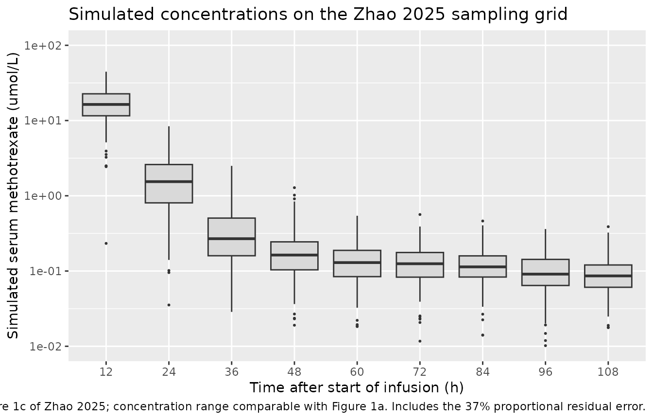

typ |>
  ggplot(aes(time, Cc, group = id, colour = arm)) +
  geom_line(alpha = 0.25) +
  scale_y_log10(limits = c(0.01, 100)) +
  scale_colour_manual(values = c("no bleomycin" = "#3b6ea5", "with bleomycin" = "#b3542f")) +
  labs(
    x = "Time after start of infusion (h)", y = "Typical-value Cc (umol/L)",
    colour = "Co-medication",
    title = "Typical-value profiles (between-subject variability zeroed)",
    caption = "Spread comes entirely from the covariate distribution and the BSA-scaled dose."
  )
#> Warning in scale_y_log10(limits = c(0.01, 100)): log-10 transformation
#> introduced infinite values.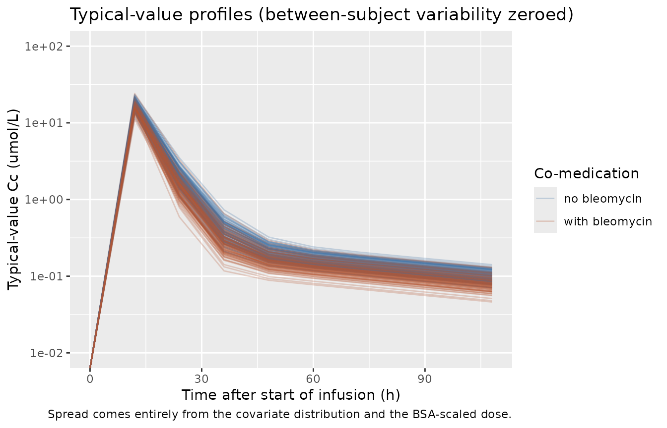

Covariate model, Equations 5 and 6

Regressing the simulated individual clearances on the covariates recovers the published exponents exactly, because the covariate model is a pure product of power terms.

# rxSolve returns the model covariates alongside the derived individual
# parameters, so one row per subject is all that is needed -- no join back to
# `cohort`, which would collide on the shared covariate column names.
per_subject <- sim |>
  group_by(id) |>
  slice(1) |>
  ungroup()

# The regression is run on the zeroRe solution, where cl and vc are exact
# deterministic functions of the covariates. Running it on the IIV-bearing
# solution would only recover the exponents to within the eta noise.
per_subject_typ <- typ |>
  group_by(id) |>
  slice(1) |>
  ungroup()

stopifnot(nrow(per_subject) == n_sub, nrow(per_subject_typ) == n_sub,
          all(c("cl", "vc", "CRCL", "WT", "TBILI", "ALB", "CONMED_BLEOMYCIN") %in%
                names(per_subject_typ)))

fit_cl <- lm(log(cl) ~ log(CRCL) + log(WT) + log(TBILI) + log(ALB) + CONMED_BLEOMYCIN,
             data = per_subject_typ)
fit_vc <- lm(log(vc) ~ log(WT), data = per_subject_typ)

recovered <- tibble(
  Term = c("eGFR on CL", "BW on CL", "TBIL on CL", "ALB on CL",
           "BLM on CL", "BW on Vc"),
  Published = c(0.23, 0.39, -0.05, -0.18, 0.08, 0.31),
  Recovered = c(
    unname(coef(fit_cl)[["log(CRCL)"]]), unname(coef(fit_cl)[["log(WT)"]]),
    unname(coef(fit_cl)[["log(TBILI)"]]), unname(coef(fit_cl)[["log(ALB)"]]),
    unname(coef(fit_cl)[["CONMED_BLEOMYCIN"]]), unname(coef(fit_vc)[["log(WT)"]])
  )
)

# Exact recovery: the covariate model is a pure product of power terms, so a
# log-log regression on the typical-value solution returns Table 3 to machine
# precision.
stopifnot(max(abs(recovered$Recovered - recovered$Published)) < 1e-8)

recovered |>
  mutate(across(c(Published, Recovered), ~ round(.x, 4))) |>
  rename("Zhao 2025 Table 3" = Published, "Recovered from simulation" = Recovered) |>
  knitr::kable(caption = "Covariate exponents recovered from the packaged model (Eqs. 5-6).")

Covariate exponents recovered from the packaged model (Eqs. 5-6).

Term	Zhao 2025 Table 3	Recovered from simulation
eGFR on CL	0.23	0.23
BW on CL	0.39	0.39
TBIL on CL	-0.05	-0.05
ALB on CL	-0.18	-0.18
BLM on CL	0.08	0.08
BW on Vc	0.31	0.31

The bleomycin term is the paper’s headline covariate finding. Zhao 2025 states that co-administration raises clearance 1.08-fold; the model reproduces exp(0.08) exactly.

# cl is a deterministic product of the covariate terms times exp(etalcl), so the
# regression coefficient on the indicator isolates the bleomycin term exactly.
blm_ratio <- exp(coef(fit_cl)[["CONMED_BLEOMYCIN"]])
stopifnot(abs(blm_ratio - exp(0.08)) < 1e-8)
sprintf("CL ratio with vs without bleomycin: %.4f (published 1.08-fold)", blm_ratio)
#> [1] "CL ratio with vs without bleomycin: 1.0833 (published 1.08-fold)"

PKNCA validation

Non-compartmental analysis is run on Cc (the individual prediction), stratified by bleomycin co-medication. Zhao 2025 reports no NCA parameters of its own, so the NCA here serves as an internal-consistency check of the packaged model against the analytic identities implied by Equations 5-8.

sim_nca <- sim |>
  filter(!is.na(Cc)) |>
  select(id, time, Cc, arm)

# Guarantee a time = 0 row per (id, arm); an intravenous infusion starting at
# time 0 has Cc = 0 there.
sim_nca <- bind_rows(
  sim_nca,
  sim_nca |> distinct(id, arm) |> mutate(time = 0, Cc = 0)
) |>
  distinct(id, arm, time, .keep_all = TRUE) |>
  arrange(id, arm, time)

conc_obj <- PKNCA::PKNCAconc(sim_nca, Cc ~ time | arm + id)

# One total-dose row per subject; the two infusion records are aggregated
# because PKNCA uses the dose only for dose-normalised parameters.
dose_df <- events |>
  filter(evid == 1) |>
  group_by(id, arm) |>
  summarise(time = 0, amt = sum(amt), .groups = "drop")

dose_obj <- PKNCA::PKNCAdose(dose_df, amt ~ time | arm + id)

intervals <- data.frame(
  start = 0, end = Inf,
  cmax = TRUE, tmax = TRUE, aucinf.obs = TRUE, auclast = TRUE, half.life = TRUE
)

nca_res <- PKNCA::pk.nca(PKNCA::PKNCAdata(conc_obj, dose_obj, intervals = intervals))

Structural identities

For a linear model with first-order elimination, AUC(0-inf) = Dose / CL holds for every individual, and the terminal half-life must equal the analytic two-compartment beta half-life computed from that subject’s own micro-constants. Both are tested per subject rather than on a cohort median, which would hide subject-level errors behind aggregation noise.

nca_wide <- as.data.frame(nca_res) |>
  select(id, arm, PPTESTCD, PPORRES) |>
  pivot_wider(names_from = PPTESTCD, values_from = PPORRES)

ident <- per_subject |>
  select(id, cl, vc, q, vp) |>
  left_join(cohort |> select(id, dose_umol), by = "id") |>
  left_join(nca_wide, by = "id") |>
  mutate(
    auc_expected = dose_umol / cl,
    auc_relerr   = abs(aucinf.obs - auc_expected) / auc_expected,
    kel = cl / vc, k12 = q / vc, k21 = q / vp,
    beta = ((kel + k12 + k21) - sqrt((kel + k12 + k21)^2 - 4 * kel * k21)) / 2,
    thalf_expected = log(2) / beta,
    thalf_relerr   = abs(half.life - thalf_expected) / thalf_expected
  )

stopifnot(
  # Both identities must be evaluable for every subject -- an NA from a failed
  # lambda-z fit would silently pass a max() with na.rm = TRUE.
  !anyNA(ident$auc_relerr),
  !anyNA(ident$thalf_relerr),
  nrow(ident) == n_sub,
  max(ident$auc_relerr)   < 0.01,   # AUC(0-inf) == Dose / CL, per subject
  max(ident$thalf_relerr) < 0.05    # terminal half-life == analytic beta half-life
)

tibble(
  Identity = c("AUC(0-inf) = Dose / CL", "t1/2,z = ln(2) / beta"),
  `Worst per-subject relative error` = sprintf(
    "%.3f%%", 100 * c(max(ident$auc_relerr), max(ident$thalf_relerr))
  )
) |>
  knitr::kable(caption = "Per-subject structural identities across all 200 simulated subjects.")

Per-subject structural identities across all 200 simulated subjects.

Identity	Worst per-subject relative error
AUC(0-inf) = Dose / CL	0.016%
t1/2,z = ln(2) / beta	0.627%

NCA summary by co-medication arm

nca_summary <- nca_wide |>
  group_by(arm) |>
  summarise(
    n = n(),
    cmax = median(cmax), tmax = median(tmax),
    aucinf.obs = median(aucinf.obs), half.life = median(half.life),
    .groups = "drop"
  )

nca_summary |>
  mutate(across(c(cmax, tmax, aucinf.obs, half.life), ~ signif(.x, 4))) |>
  rename(
    "Co-medication"          = arm,
    "N"                      = n,
    "Cmax (umol/L)"          = cmax,
    "Tmax (h)"               = tmax,
    "AUC0-inf (umol*h/L)"    = aucinf.obs,
    "t1/2,z (h)"             = half.life
  ) |>
  knitr::kable(caption = "Simulated NCA medians by bleomycin co-medication arm.")

Simulated NCA medians by bleomycin co-medication arm.

Co-medication	N	Cmax (umol/L)	Tmax (h)	AUC0-inf (umol*h/L)	t1/2,z (h)
no bleomycin	76	18.43	12	325.9	66.39
with bleomycin	124	17.71	1	289.3	65.75

The median Tmax differs between the arms, and that is a real consequence of the protocol’s split infusion rather than an artefact. One third of the dose goes in over 1 h and the remaining two thirds over 11 h, so the first hour runs at about 5.5 times the rate of the following eleven. The profile therefore has two nearly equal peaks – one at the end of the fast infusion (1 h) and one at the end of the slow infusion (12 h) – and which is higher depends on the subject’s own CL/Vc ratio. Raising clearance depresses the long infusion’s plateau more than the short infusion’s spike, so the with-bleomycin arm tips towards the 1 h peak.

Bleomycin raises clearance, so the with-bleomycin arm should show a lower median AUC than the no-bleomycin arm once the arms are matched on dose. Because the two virtual arms differ in BSA-scaled dose by chance, the comparison below is made on dose-normalised AUC.

auc_norm <- ident |>            # `arm` already rode in from the PKNCA grouping
  group_by(arm) |>
  summarise(`Median dose-normalised AUC (h/L)` = median(aucinf.obs / dose_umol),
            .groups = "drop")

stopifnot(
  auc_norm$`Median dose-normalised AUC (h/L)`[auc_norm$arm == "with bleomycin"] <
    auc_norm$`Median dose-normalised AUC (h/L)`[auc_norm$arm == "no bleomycin"]
)

auc_norm |>
  mutate(`Median dose-normalised AUC (h/L)` = signif(`Median dose-normalised AUC (h/L)`, 4)) |>
  rename("Co-medication" = arm) |>
  knitr::kable(caption = "Dose-normalised exposure is lower with bleomycin, as the positive CL coefficient requires.")

Dose-normalised exposure is lower with bleomycin, as the positive CL coefficient requires.

Co-medication	Median dose-normalised AUC (h/L)
no bleomycin	0.08097
with bleomycin	0.07312

Comparison against published values

Zhao 2025 reports no non-compartmental parameters, so nlmixr2lib::ncaComparisonTable() has nothing to compare against. The table below instead pairs every published quantitative anchor in the paper with its simulated counterpart.

typ_ref <- rxode2::rxSolve(
  mod_typical,
  events = tibble(
    id = 1L, time = c(0, 0, 1, 12), evid = c(1L, 0L, 1L, 0L),
    amt = c(1000, NA_real_, 2000, NA_real_),
    dur = c(1, NA_real_, 11, NA_real_), cmt = "central",
    CRCL = 102.2, WT = 47, TBILI = 15.3, ALB = 40.9, CONMED_BLEOMYCIN = 0
  ),
  omega = NA, sigma = NA
) |>
  as.data.frame()

pooled <- sim_tdm_realistic$sim

anchors <- tibble(
  Quantity = c(
    "Typical CL at the reference covariate set (L/h)",
    "Typical Vc at 47 kg (L)",
    "Q, fixed (L/h)",
    "Vp, fixed (L)",
    "CL fold-change with concomitant bleomycin",
    "Pooled MTX concentration, median (umol/L)",
    "Pooled MTX concentration, minimum (umol/L)",
    "Pooled MTX concentration, maximum (umol/L)"
  ),
  `Zhao 2025` = c("12.88", "72.04", "1.08", "94.94", "1.08",
                  "1.2", "0.01", "55.80"),
  Source = c("Table 3 / Eq. 5", "Table 3 / Eq. 6", "Table 3 / Eq. 7",
             "Table 3 / Eq. 8", "Abstract; Discussion",
             "Table 1", "Table 1", "Table 1"),
  Simulated = c(
    sprintf("%.2f", typ_ref$cl[1]),
    sprintf("%.2f", typ_ref$vc[1]),
    sprintf("%.2f", typ_ref$q[1]),
    sprintf("%.2f", typ_ref$vp[1]),
    sprintf("%.2f", blm_ratio),
    sprintf("%.2f", median(pooled)),
    sprintf("%.3f", min(pooled)),
    sprintf("%.2f", max(pooled))
  )
)

# The four structural parameters and the bleomycin ratio are exact identities.
stopifnot(
  abs(typ_ref$cl[1] - 12.88) < 1e-6,
  abs(typ_ref$vc[1] - 72.04) < 1e-6,
  abs(typ_ref$q[1]  - 1.08)  < 1e-6,
  abs(typ_ref$vp[1] - 94.94) < 1e-6
)
# The pooled concentration distribution must sit inside the Table 1 envelope and
# put its median within a factor of about two of the reported 1.2 umol/L. Exact
# agreement is not reachable: every simulated subject receives the protocol
# standard 1.3 g/m^2 whereas the real cohort only had to exceed 0.5 g/m^2, and
# the realised dose distribution is never reported. That biases the simulated
# distribution upwards.
stopifnot(
  median(pooled) > 0.6, median(pooled) < 2.5,
  max(pooled) < 55.80,
  min(pooled) > 0.001
)

knitr::kable(
  anchors,
  caption = "Every quantitative anchor published in Zhao 2025 against its simulated counterpart.",
  align = c("l", "r", "l", "r")
)

Every quantitative anchor published in Zhao 2025 against its simulated counterpart.

Quantity	Zhao 2025	Source	Simulated
Typical CL at the reference covariate set (L/h)	12.88	Table 3 / Eq. 5	12.88
Typical Vc at 47 kg (L)	72.04	Table 3 / Eq. 6	72.04
Q, fixed (L/h)	1.08	Table 3 / Eq. 7	1.08
Vp, fixed (L)	94.94	Table 3 / Eq. 8	94.94
CL fold-change with concomitant bleomycin	1.08	Abstract; Discussion	1.08
Pooled MTX concentration, median (umol/L)	1.2	Table 1	0.81
Pooled MTX concentration, minimum (umol/L)	0.01	Table 1	0.018
Pooled MTX concentration, maximum (umol/L)	55.80	Table 1	44.59

For orientation, the Discussion compares this model with the two-compartment methotrexate model of Nader 2017 (CL 15.7 L/h, Vc 79.2 L, Q 0.97 L/h, Vp 51.4 L) and notes that “except for the typical value of Vp, which slightly falls outside the range of previous studies (51.4 L vs. 94.94 L), all other parameters were within the ranges of earlier models”.

Assumptions and deviations

• The scale of the two IIV rows in Table 3 is ambiguous as printed, and is resolved here by a variance-decomposition identity internal to the paper. Table 3 labels its variability rows IIV Vc(CV%) and IIV CL(CV%) and prints 0.32 and 2.98 for the final model (1.20 and 5.07 for the base model), with no RSE and no confidence interval on either row. The % in the header cannot be taken at face value, because the same table’s (%RSE) column verifiably holds fractions rather than percents: on all nine rows that carry a confidence interval, the CI-implied relative standard error reproduces the printed value only when read as a fraction (Vc 72.04 with CI 70.00-74.09 gives RSE 0.0145, printed 0.01; TBIL -0.05 with CI -0.07 to -0.02 gives RSE -0.255, printed -0.27). Four readings are therefore on the table: the value is a CV in percent, a CV as a fraction, omega^2 x 100, or omega^2.

  The paper settles it. A covariate model can only explain variability that the base model’s IIV actually contained, so omega^2(base) - omega^2(final) must be about equal to the variance the retained covariates inject into the parameter, and that quantity is computable from the Table 1 covariate ranges and the Eq. 5-6 exponents. Treating the Table 1 ranges as +-3.1 SD of a log-normal (n = 505), the covariates inject var(log CL) = 0.0286 and var(log Vc) = 0.0116:

  Reading of the printed value	Drop in CL	Ratio	Drop in Vc	Ratio
  CV in percent	0.00168	0.06	0.00013	0.01
  CV as a fraction	0.99429	34.77	0.79451	68.32
  omega^2 x 100	0.02090	0.73	0.00880	0.76
  omega^2	2.09000	73.10	0.88000	75.67

  Only omega^2 x 100 is the right order of magnitude, and it lands on the same ratio for CL and for Vc (0.73 and 0.76) even though the two parameters carry different covariate structures – a coincidence a wrong scale factor would not produce. The shared shortfall below 1.0 is what collinearity among BW, BSA and eGFR plus the range-to-SD conversion would predict. The other three readings miss by factors of 17 to 75. The visual predictive check (Figure 2) agrees: simulated 5th-to-95th percentile spans under this reading are about 1.2 decades against roughly 1.3 decades read off the published figure, whereas the “CV as a fraction” and “omega^2” readings both give more than 4 decades, and the “CV in percent” reading is indistinguishable from a model with no IIV at all.

  The model file therefore encodes omega^2 = printed/100: etalcl ~ 0.0298 (CV 17.4%) and etalvc ~ 0.0032 (CV 5.7%). The base-model values then correspond to CVs of 22.8% and 11.0%, with the covariates absorbing the difference. These magnitudes are also in line with published methotrexate population PK models. This is an inference about the reporting scale, not a value printed in the paper, so anyone re-fitting the model should re-derive it.

• Sampling times are taken from Figure 1c, not from the Methods text. Methods 2.3 says blood was collected “24 h after the completion of each MTX infusion, followed by sampling at 12-h intervals up to a maximum of 108 h”, which would place the first sample at 36 h given the 12 h infusion. The x-axis of the Figure 1c goodness-of-fit panel instead shows dense observation stripes beginning at approximately 12 h after dose and repeating every 12 h to about 108 h, and the Discussion refers to record availability “at 48 h, 60 h and 72 h” in a day-relative sense consistent with timing from the start of dosing. The simulated grid follows the figure (12, 24, …, 108 h from the start of the infusion). The choice affects only which concentrations the figures display; it does not touch any model parameter.

• Cohort covariate distributions are reconstructed from marginals. Table 1 reports medians and ranges only, with no standard deviations and no correlation structure. Body weight, eGFR and total bilirubin are drawn log-normally, and albumin normally, with dispersion chosen so the simulated ranges cover the reported ranges; all are clamped to those ranges. Height is derived from weight by a power relation anchored on the Table 1 median pair, and BSA follows from the Mosteller equation the paper used. eGFR, bilirubin and albumin are drawn independently of weight; in the real cohort they are certainly correlated with body size, particularly eGFR in a cohort that is 73.3% children.

• Dose held at the protocol standard. Methods 2.1 gives a standard dose of 1.3 g/m^2 while the inclusion criterion is only “>= 0.5 g/m^2”, and the paper never reports the realised dose distribution. Every simulated subject receives 1.3 g/m^2. This inflates the simulated concentration distribution relative to the pooled Table 1 statistics, which is the main reason the pooled-median comparison is given a loose tolerance.

• Record availability over the sampling grid is reconstructed. The pooled concentration statistics can only be compared with Table 1 if the simulated records are distributed over the sampling grid the way the real ones are, and they are not distributed evenly: the Discussion states that records were “available for 53.07% at 48 h, 26.53% at 60 h, and only 1.39% at 72 h”. Those three percentages are used directly; the three earlier times (12, 24, 36 h) are assumed complete, which is what the Figure 1c stripe densities show but is not stated numerically. Times past 72 h are excluded from the pooled statistics because the paper gives no availability for them; they still appear in the concentration-time figure.

• A proportional error model on the linear scale can draw negative concentrations. Methods 2.5.1 Eq. 3 gives the residual model as C_obs = C_pred * (1 + epsilon) with a 37% standard deviation, which produces a negative simulated concentration whenever epsilon < -1. No assay can report one, so those draws are discarded before the pooled statistics are computed (the vignette asserts the discarded fraction stays under 2%). This is a property of the published error model, not of the extraction.

• Molar conversion uses an external constant. The paper reports doses in g/m^2 and concentrations in umol/L but never states the molecular weight used. The vignette converts with 454.44 g/mol (methotrexate, PubChem CID 126941). This constant is used only inside the vignette to build the event table; it is not a model parameter and does not appear in the model file.

• Non-compartmental comparison is internal. The paper publishes no Cmax, Tmax, AUC or half-life, so there is nothing to compare the PKNCA output against externally. The NCA section instead asserts the analytic identities the model must satisfy (AUC(0-inf) = Dose / CL and the two-compartment beta half-life) per subject, and the published-anchor table covers every numeric value the paper does report.

• Sex is inconsistently reported in the source. Table 1 gives “Sex (Male/Female) 357/148” while Results 3.1 gives “505 patients (357 females and 148 males)”. Sex is not a covariate in the final model, so the discrepancy has no effect on any equation; the population metadata follows the Table 1 column header and records the conflict.

• Concomitant-medication percentages have an ambiguous denominator. Table 1 lists bleomycin as “941 (58.67%)” under “Concomitant medications”, and 941 is 58.67% of about 1,604 records rather than of the 505 patients, yet Results 3.1 states that “concurrent use of BLM was observed in 58.67% of patients”. The virtual cohort assigns bleomycin to 58.67% of subjects, following the Results sentence.

• No supplement, erratum or correction was found. A search of the Frontiers in Pharmacology article landing page and of PubMed for corrections to doi:10.3389/fphar.2025.1548203 returned nothing as of the extraction date; all values come from the main text.