Pacmilimab conditionally activated anti-PD-L1 TNBC QSP (Ippolito 2024)
Source:vignettes/articles/Ippolito_2024_pacmilimab_qsp.Rmd
Ippolito_2024_pacmilimab_qsp.RmdModel and source
# built once and reused throughout: this is a 240-state model and each build
# costs about a minute
mod <- rxode2::rxode2(readModelDb("Ippolito_2024_pacmilimab_qsp"))
length(mod$state)
#> [1] 240- Citation: Ippolito A, Wang H, Zhang Yu, Vakil V, Bazzazi H, Popel AS. Eliciting the antitumor immune response with a conditionally activated PD-L1 targeting antibody analyzed with a quantitative systems pharmacology model. CPT Pharmacometrics Syst Pharmacol. 2024;13(1):93-105. doi:10.1002/psp4.13060. Structure of the inherited QSP-IO platform from the SimBiology export in Wang H, Zhao C, Santa-Maria CA, Emens LA, Popel AS. Dynamics of tumor-associated macrophages in a quantitative systems pharmacology model of immunotherapy in triple-negative breast cancer. iScience. 2022;25(8):104702. doi:10.1016/j.isci.2022.104702.
- Article: https://doi.org/10.1002/psp4.13060
- Appendix S1 (Eqs S1-S68) and Tables S1-S2: supporting information of the article
Pacmilimab is a Probody therapeutic (PbTx): an anti-PD-L1 antibody
whose two active sites are each covered by a mask held on by a
protease-cleavable linker. The mask shifts reversibly to reveal the
active site (equilibrium constant K_M), and is removed
irreversibly by tumour-associated proteases (rate k_cvg),
which are far more active inside the tumour than outside it. The paper
embeds this dynamic in the Popel-laboratory QSP-IO platform previously
validated for atezolizumab in triple-negative breast cancer, and adds an
out-of-synapse module so PD-L1 outside the immunological synapse can
also bind drug.
This is a deterministic mechanism model, not a population model. The authors generate virtual patients by Latin hypercube sampling of the 29 parameter distributions in Supplementary Table S1; there are no etas and no residual error model, so everything below is a typical-value simulation.
Population
| Field | Value |
|---|---|
| species | human (in silico virtual cohort) |
| n_subjects | 10000 |
| disease_state | triple-negative breast cancer |
| dose_range | Pacmilimab 10 mg/kg every 2 weeks for 400 days is the reference regimen (the schedule selected in the phase I trial); the paper additionally explores 1, 3, 10 and 15 mg/kg at q1w, q2w, q3w and q4w, and single doses of 0.1, 0.3, 1, 3 and 10 mg/kg for the PK calibration. |
| notes | Virtual cohort of 10,000 patients generated by Latin hypercube sampling of the 29 parameter distributions in Supplementary Table S1, then pruned to plausible patients. Each patient is grown from a small cancer-cell population to the pre-treatment tumour size before dosing starts. The clinical anchors are the pacmilimab phase I trial (16 patients with TNBC, objective response rate 7%) and the single-dose PK of Stroh 2021. |
The clinical anchors are the pacmilimab phase I study (16 patients with TNBC, objective response rate 7%) and the single-dose PK of Stroh 2021 at 0.1, 0.3, 1, 3 and 10 mg/kg. The regimen selected in that trial, and simulated throughout the paper, is 10 mg/kg every two weeks for 400 days.
Model structure
| Layer | Content |
|---|---|
| Physiological compartments | central, peripheral, tumour, tumour-draining lymph node |
| Antigen-presentation compartments | APC endosome (V_e), APC surface (A_s,
A_e) |
| Synapse compartments | T cell-cancer cell, T cell-APC, macrophage-cancer cell |
| Out-of-synapse compartments (new in this paper) | cancer cell, T cell, macrophage, APC |
| Cell populations | two cancer clones, naive/activated/effector CD8 and CD4 T cells, Tregs, exhausted T cells, APC and mature APC, MDSC, M1 and M2 macrophages |
| Soluble mediators | IL-2, IL-10, IL-12, IFN-gamma, TGF-beta, CCL2, nitric oxide, arginase-I, angiogenic factor |
| Checkpoints | PD-1/PD-L1/PD-L2, CTLA-4/CD28/CD80/CD86, CD47/SIRP-alpha |
| Probody | six free states per compartment, nine bound states at each of nine PD-L1 bearing sites |
States are integrated as amounts
(q_<compartment>_<species>) and the
declared-unit value (concentration, surface density or cell count) is
derived algebraically as
x_<compartment>_<species>. This is what
SimBiology does internally and it removes the dilution question for the
tumour compartment, whose volume vol_V_T is a
state-dependent repeated assignment over the cell counts it
contains.
The six free Probody states are named for the status of the two
active sites: m masked, o open (mask present
but revealing the site), c cleaved. So P_mm is
fully masked (the form injected as pacmilimab), P_cc is
fully cleaved (equivalent to the naked anti-PD-L1 antibody), and
P_co has one site cleaved and one open. Per Figure 4a of
the paper, the active states are every state except
P_mm.
Source trace
| Model element | Source |
|---|---|
| Probody state transitions (unmasking, cleavage), 4 compartments | Ippolito Appendix S1 Eqs S51-S56 |
| Probody transport and central clearance | Ippolito Appendix S1 Eqs S30-S33 |
| Probody mono- and bivalent PD-L1 binding, 9 states per site | Ippolito Appendix S1 Eqs S57-S65 |
| Out-of-synapse PD-L1 binding and turnover, 4 compartments | Ippolito Appendix S1 Eqs S66-S68 |
Unmasking equilibrium K_M = 1/175, unmasking rate
k_o = 0.0116 /s |
Ippolito Table S2 |
Cleavage rate k_cvg = 1e-07 /s (tumour) |
Ippolito Table S1, “Probody cleavage rate in TNBC” |
| Extra-tumoral cleavage = 1% of the tumour rate | Ippolito Appendix S1, “Model implementation” |
| All 237 remaining parameter values | Ippolito Table S2 |
| Cancer, T cell, APC, antigen, checkpoint, MDSC and macrophage ODEs | Wang 2022 iScience Tables S3-S6 (the SimBiology export of the platform this paper inherits, cited as ref. 3 of Appendix S1) |
kon_CD80_CD80, koff_CD80_CD80
|
Wang 2022 Table S2 (absent from Ippolito Table S2; see Errata) |
| Antibody molar mass 145 kDa | Wang 2022 supplementary methods (atezolizumab; the paper assumes the PbTx shares its PK) |
Every parameter carries an inline comment in the model file naming its source table and its value in the source’s own units, alongside the converted value used by the model.
MW <- 145000                                   # g/mol, 145 kDa
WT <- 70                                       # kg (not reported; see Errata)
nmol_of <- function(mgkg) mgkg * WT / MW * 1e6
diam_cm <- function(v_L) (6 * v_L * 1000 / pi)^(1/3)
# rtol 1e-7 reproduces rtol 1e-8 to 7-8 significant figures on every quantity
# used below, at ~200x less cost on the stiff early growth phase
SOLVE <- list(atol = 1e-10, rtol = 1e-7, maxsteps = 1e7)
solv <- function(...) do.call(rxode2::rxSolve,
  c(list(mod, ...), SOLVE, list(returnType = "data.frame")))

FREE   <- c("P_mm", "P_mo", "P_oo", "P_cm", "P_co", "P_cc")
ACTIVE <- setdiff(FREE, "P_mm")                # Figure 4a
UNCLEAVED <- c("P_mm", "P_mo", "P_oo")         # Figure 2b assay
Initialisation: untreated tumour growth
The paper’s virtual-patient protocol simulates each patient from a small cancer-cell population until the tumour reaches the pre-treatment size, then starts dosing. Table S1 gives a median pre-treatment diameter of 2.5 cm.
grow <- solv(rxode2::et(seq(0, 320, by = 5)))
grow$diam <- diam_cm(grow$vol_V_T)
day_start <- grow$time[which.min(abs(grow$diam - 2.5))]
day_start
#> [1] 275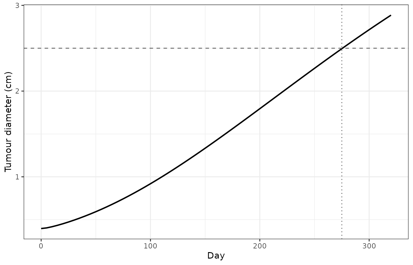
Untreated Gompertzian growth from the Table S3 initial cancer-cell population to the 2.5 cm median pre-treatment diameter of Table S1.
The state at that point is the pre-treatment patient used for every arm below.
ref <- grow[which.min(abs(grow$diam - 2.5)), ]
inits <- unlist(ref[mod$state]); names(inits) <- mod$state
inits[inits < 0] <- 0| Quantity | Value |
|---|---|
| H_PD1_C1 | 0.998690 |
| H_PD1_APC | 0.998860 |
| H_CD28_APC | 0.949160 |
| H_APC | 0.999690 |
| H_P0 | 0.049391 |
| H_P1 | 0.454120 |
| H_TGFb | 0.353500 |
| H_MDSC | 0.432270 |
| H_IL10 | 0.118150 |
| H_IL12 | 0.816460 |
| H_SIRPa | 0.877550 |
| H_PD1_M | 0.549690 |
| H_Mac_C | 0.944860 |
| N_aT | 12.102000 |
| N_aT0 | 10.453000 |
| Teff/Treg | 2.070800 |
| M1/M2 | 0.481060 |
Unlike the sibling Anbari 2023 export, Ippolito’s Table S2 stores
SimBiology’s default values for the repeated-assignment targets
(H_APC 0.5, H_PD1_C1 0.9, N_aT 1,
C_total 0) rather than converged reference-state outputs,
so this table is a description of the model’s own pre-treatment state
rather than a check against published numbers. Those rows are model
outputs and are deliberately not carried into
ini(); see Errata.
Probody mass conservation
Two conservation identities follow from Eqs S51-S65 and hold independently of any parameter value, so they are the sharpest available test that the Probody equations were transcribed correctly.
Free states. Unmasking and cleavage only move drug between the six free states and transport only moves it between compartments, so free drug plus cumulative central clearance must equal the dose at all times. Note that free drug is deliberately not decremented by surface binding: Appendix S1 assumes “an abundance of probody and antibody in each compartment compared to the ones interacting with the cell surface”, exactly as the parent model’s own aPDL1 reactions do. Free-plus-bound is therefore not a conserved quantity.
mk_ev <- function(target, amt, grid, ii = NULL, addl = NULL) {
  d <- if (is.null(ii)) rxode2::et(amt = amt, time = 0, cmt = target)
       else rxode2::et(amt = amt, time = 0, cmt = target, ii = ii, addl = addl)
  rxode2::add.sampling(d, grid)
}
dose10 <- nmol_of(10)
pk_grid <- seq(0, 84, by = 0.25)
pk_pb <- solv(mk_ev("q_V_C_P_mm", dose10, pk_grid), inits = inits)

free_drug <- function(s) rowSums(s[, as.vector(outer(c("V_C", "V_P", "V_T", "V_LN"),
  FREE, function(a, b) paste0("q_", a, "_", b))), drop = FALSE])
clear_rate <- function(s) rowSums(s[, paste0("vpb_cl_", FREE), drop = FALSE])
cum_trap <- function(t, y) c(0, cumsum(diff(t) * (head(y, -1) + tail(y, -1)) / 2))

bal <- free_drug(pk_pb) + cum_trap(pk_pb$time, clear_rate(pk_pb))
max(abs(bal / dose10 - 1))
#> [1] 0.0001961778
stopifnot(max(abs(bal / dose10 - 1)) < 1e-3)
Bound states. With association switched off, the
cleavage and unmasking terms of Eqs S57-S65 must cancel exactly, leaving
dissociation of the monovalent complexes as the only sink. (A bivalent
complex that loses one bond becomes a monovalent complex, so its
2*koff term is a transfer within the bound pool, not a sink
from it.)
BOUND <- c("P_mo_fb", "P_oo_fb", "P_cm_bf", "P_co_bf", "P_co_fb", "P_cc_fb",
           "P_oo_bb", "P_co_bb", "P_cc_bb")
site <- "syn_T_C1_PDL1"
i2 <- inits
for (b in BOUND) i2[[paste0("q_", site, "_", b)]] <- 1
bs <- solv(rxode2::et(seq(0, 0.4, by = 0.001)), inits = i2,
           params = c(kon_PDL1_aPDL1 = 0))
mono <- rowSums(bs[, paste0("q_", site, "_", BOUND[1:6]), drop = FALSE])
biv  <- rowSums(bs[, paste0("q_", site, "_", BOUND[7:9]), drop = FALSE])
tot  <- mono + biv
k    <- which(tot > 1e-6); k <- k[k > 1 & k < length(tot)]
dtot <- (tot[k + 1] - tot[k - 1]) / (bs$time[k + 1] - bs$time[k - 1])
pred <- (-bs$p_koff_PDL1_aPDL1[1] * mono)[k]
max(abs((dtot - pred) / pred))
#> [1] 7.102085e-05
stopifnot(max(abs((dtot - pred) / pred)) < 1e-3)
Both identities hold to solver tolerance. The second one is what caught three defects in the printed equations (see Errata) - it fails on five states if Eqs S61 and S62 are implemented exactly as printed.
Antibody pharmacokinetics
Figure 2b of the paper calibrates the model against single-dose blood
concentrations of uncleaved pacmilimab at 0.1, 0.3, 1,
3 and 10 mg/kg. Uncleaved means no site has been cleaved,
i.e. P_mm + P_mo + P_oo.
doses <- c(0.1, 1, 10)
pk <- lapply(doses, function(d) {
  s <- solv(mk_ev("q_V_C_P_mm", nmol_of(d), pk_grid), inits = inits)
  data.frame(id = 1L, treatment = paste0(d, " mg/kg"), dose_mgkg = d,
             time = s$time,
             Cc = rowSums(s[, paste0("q_V_C_", UNCLEAVED), drop = FALSE]) / s$m_V_C)
}) |> bind_rows()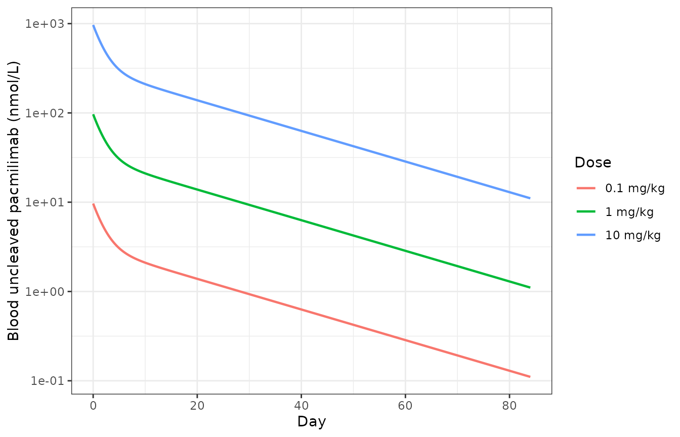
Replicates Figure 2b of Ippolito 2024: simulated blood uncleaved pacmilimab after a single dose.
Non-compartmental analysis of the simulated profiles
conc_df <- pk |> dplyr::filter(!is.na(Cc))
dose_df <- pk |>
  dplyr::distinct(id, treatment, dose_mgkg) |>
  dplyr::mutate(time = 0, amt = nmol_of(dose_mgkg))
o_conc <- PKNCA::PKNCAconc(conc_df, Cc ~ time | treatment / id)
o_dose <- PKNCA::PKNCAdose(dose_df, amt ~ time | treatment + id,
                           route = "intravascular", duration = 0)
# one explicit interval spanning the whole profile, so every parameter comes
# from the same interval (PKNCA's default puts auclast on 0-24 h and the rest
# on 0-Inf, which would mix intervals in the table below)
ivl <- data.frame(start = 0, end = max(pk_grid), cmax = TRUE, tmax = TRUE,
                  auclast = TRUE, aucinf.obs = TRUE, half.life = TRUE, cl.obs = TRUE)
res_nca <- PKNCA::pk.nca(PKNCA::PKNCAdata(o_conc, o_dose, intervals = ivl))| treatment | auclast | cmax | tmax | half.life | aucinf.obs | cl.obs | dose_mgkg |
|---|---|---|---|---|---|---|---|
| 0.1 mg/kg | 87.75 | 9.655 | 0 | 17.47 | 90.53 | 0.5332 | 0.1 |
| 1 mg/kg | 877.50 | 96.550 | 0 | 17.47 | 905.30 | 0.5332 | 1.0 |
| 10 mg/kg | 8775.00 | 965.500 | 0 | 17.47 | 9054.00 | 0.5332 | 10.0 |
The paper publishes no NCA table for pacmilimab, so there are no reference values to compare against. What is checkable is that the free-Probody sub-system is strictly linear - drug appears in the transport, unmasking and cleavage terms only as a first-order reactant, and surface binding does not consume it - so every exposure metric must be exactly dose-proportional.
spread <- function(x) max(x) / min(x) - 1
lin <- nca_raw |>
  dplyr::mutate(cmax_per_mgkg = cmax / dose_mgkg,
                auclast_per_mgkg = auclast / dose_mgkg,
                aucinf_per_mgkg = aucinf.obs / dose_mgkg)
c(cmax = spread(lin$cmax_per_mgkg),
  auclast = spread(lin$auclast_per_mgkg),
  aucinf = spread(lin$aucinf_per_mgkg),
  half.life = spread(lin$half.life),
  cl.obs = spread(lin$cl.obs))
#>         cmax      auclast       aucinf    half.life       cl.obs
#> 0.000000e+00 6.737303e-07 6.387542e-07 2.182133e-07 6.387542e-07
stopifnot(
  spread(lin$cmax_per_mgkg) < 1e-8,
  spread(lin$auclast_per_mgkg) < 1e-5,
  spread(lin$aucinf_per_mgkg) < 1e-5,
  spread(lin$half.life) < 1e-5,
  spread(lin$cl.obs) < 1e-5
)
Dose-normalised Cmax, AUClast and
AUCinf, the terminal half-life and the clearance are
identical across a 100-fold dose range, as they must be.
Only a small fraction of the dose is cleaved systemically, which is the direct consequence of the paper’s assumption that extra-tumoral cleavage runs at 1% of the tumour rate:
Treatment comparison
The paper simulates three arms over 400 days: untreated, unmasked
anti-PD-L1 monotherapy, and pacmilimab monotherapy, all at 10 mg/kg
every two weeks. The unmasked arm is produced by dosing the fully
cleaved state P_cc - Appendix S1 defines it as “injecting a
fully cleaved (i.e., without both masks) antibody” - so a single model
covers all three arms.
tr_grid <- seq(0, 400, by = 5)
arm <- function(target) solv(mk_ev(target, dose10, tr_grid, ii = 14, addl = 28),
                             inits = inits)
untreated <- solv(rxode2::et(tr_grid), inits = inits)
unmasked  <- arm("q_V_C_P_cc")
pbtx      <- arm("q_V_C_P_mm")

arms <- bind_rows(
  data.frame(arm = "untreated",  time = untreated$time, vol = untreated$vol_V_T,
             H_PD1 = untreated$H_PD1_C1),
  data.frame(arm = "unmasked",   time = unmasked$time,  vol = unmasked$vol_V_T,
             H_PD1 = unmasked$H_PD1_C1),
  data.frame(arm = "pacmilimab", time = pbtx$time,      vol = pbtx$vol_V_T,
             H_PD1 = pbtx$H_PD1_C1)) |>
  group_by(arm) |>
  mutate(diam = diam_cm(vol), pct_change = 100 * (vol / first(vol) - 1)) |>
  ungroup()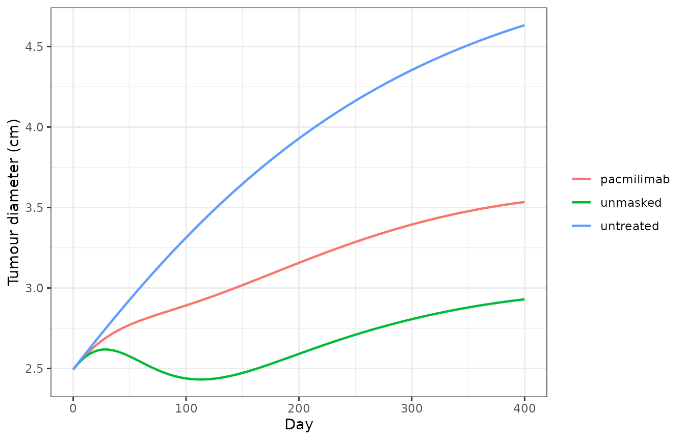
Replicates the tumour-size comparison of Figure 3 of Ippolito 2024 for the typical patient: pacmilimab is intermediate between the untreated and unmasked arms.
| Arm | Diameter day 0 (cm) | Diameter day 400 (cm) | Volume change (%) |
|---|---|---|---|
| pacmilimab | 2.495 | 3.534 | 184.40 |
| unmasked | 2.495 | 2.930 | 61.99 |
| untreated | 2.495 | 4.633 | 540.50 |
final <- arms |> group_by(arm) |> summarise(v = last(vol), .groups = "drop")
stopifnot(
  final$v[final$arm == "unmasked"] < final$v[final$arm == "pacmilimab"],
  final$v[final$arm == "pacmilimab"] < final$v[final$arm == "untreated"]
)
The ordering reproduces the paper’s central efficacy conclusion: masking costs some efficacy, but both antibodies are far better than no treatment. Figure S1 of the paper shows the corresponding fall in the PD-1 checkpoint Hill term, and the same ordering appears here.
| Arm | H_PD1 at day 400 |
|---|---|
| pacmilimab | 0.43615 |
| unmasked | 0.30319 |
| untreated | 0.99856 |
Tumour selectivity of activation
Figure 4 of the paper compares the concentration of active antibody (any state with at least one open or cleaved site) between compartments, and reports that masking raises the tumour-to-periphery and tumour-to-blood ratios by roughly 10% while dropping the absolute peripheral exposure by more than an order of magnitude.
act_conc <- function(s, cp) {
  cap <- if (cp == "V_T") s$vol_V_T else s[[paste0("m_", cp)]]
  rowSums(s[, paste0("q_", cp, "_", ACTIVE), drop = FALSE]) / cap
}
act_frac <- function(s, cp) rowSums(s[, paste0("q_", cp, "_", ACTIVE), drop = FALSE]) /
                            rowSums(s[, paste0("q_", cp, "_", FREE), drop = FALSE])

sel <- data.frame(
  Arm = c("unmasked", "pacmilimab"),
  `Active in tumour (nmol/L)`     = c(tail(act_conc(unmasked, "V_T"), 1),
                                      tail(act_conc(pbtx, "V_T"), 1)),
  `Active in periphery (nmol/L)`  = c(tail(act_conc(unmasked, "V_P"), 1),
                                      tail(act_conc(pbtx, "V_P"), 1)),
  `Active fraction, tumour`       = c(tail(act_frac(unmasked, "V_T"), 1),
                                      tail(act_frac(pbtx, "V_T"), 1)),
  `Active fraction, periphery`    = c(tail(act_frac(unmasked, "V_P"), 1),
                                      tail(act_frac(pbtx, "V_P"), 1)),
  `Active fraction, blood`        = c(tail(act_frac(unmasked, "V_C"), 1),
                                      tail(act_frac(pbtx, "V_C"), 1)),
  check.names = FALSE)
sel$`Selectivity T/P` <- sel$`Active fraction, tumour` / sel$`Active fraction, periphery`
sel$`Selectivity T/blood` <- sel$`Active fraction, tumour` / sel$`Active fraction, blood`| Arm | Active in tumour (nmol/L) | Active in periphery (nmol/L) | Active fraction, tumour | Active fraction, periphery | Active fraction, blood | Selectivity T/P | Selectivity T/blood |
|---|---|---|---|---|---|---|---|
| unmasked | 95.730 | 73.800 | 1.00000 | 1.00000 | 1.00000 | 1.000 | 1.000 |
| pacmilimab | 1.169 | 1.185 | 0.01952 | 0.01605 | 0.01596 | 1.216 | 1.223 |
periph_fold <- sel$`Active in periphery (nmol/L)`[1] / sel$`Active in periphery (nmol/L)`[2]
periph_fold
#> [1] 62.30262
stopifnot(
  periph_fold > 10,                       # paper: "more than an order of magnitude"
  sel$`Selectivity T/P`[2] > 1.10,        # masking concentrates activation in the TME
  sel$`Selectivity T/blood`[2] > 1.10,
  abs(sel$`Selectivity T/P`[1] - 1) < 1e-9  # the unmasked antibody is active everywhere
)
The active fraction of circulating pacmilimab is about 2%, and it is roughly 22% higher inside the tumour than in the periphery or the blood - the conditional-activation effect the molecule is designed for. The unmasked antibody is by construction 100% active in every compartment, so its selectivity is exactly 1. Absolute active exposure in the periphery is 62.3-fold lower for pacmilimab, comfortably reproducing the paper’s “more than an order of magnitude” claim.
Note that the raw concentration ratio
[A]_T/[A]_P plotted in Figures 4b and 4d is not reproduced
in the same direction at typical-value parameters, because the two arms
end the 400 days with different tumour volumes and the tumour
concentration is diluted accordingly. The paper averages that ratio over
10,000 virtual patients, where the between-arm difference in tumour size
is much smaller. The volume-free active-fraction comparison above
isolates the mechanism the paper is describing and does reproduce
it.
Assumptions and deviations
- Antibody molar mass and body weight. Doses are reported in mg/kg. The molar mass is not given for pacmilimab; the model assumes the 145 kDa of atezolizumab reported in the Wang 2022 supplementary methods, consistent with the paper’s own statement that the PbTx shares atezolizumab’s PK. Body weight is not reported anywhere; 70 kg is used. Both only set the scale of the dose in nmol: the free-Probody sub-system is exactly linear, so every ratio, fraction and dose-normalised metric in this vignette is invariant to them.
-
Three defects in the printed Probody equations.
Requiring that cleavage and dissociation conserve antibody across Eqs
S57-S65 determines all three uniquely:
- Eq S61 loses
k_cvg [P_co,bf]; it must bek_cvg [P_co,fb], otherwiseP_co,fbhas no cleavage sink andP_co,bfhas two. - Eq S61 gains
koff [P_oo,bb]; it must bekoff [P_co,bb], sinceP_oo,bbalready returns2*kofftoP_oo,fbin Eq S58 while the2*koffsink ofP_co,bbin Eq S64 is otherwise unmatched. - Eq S62 carries a dangling
+ k_cvgwith no species and writes its own dissociation sink askoff [P_co,fb]. The dangling term isk_cvg [P_cm,bf]- the only cleavage flux in Eq S59 with no destination - and the sink iskoff [P_cc,fb]. The bound-state conservation check above fails on five states without these corrections.
- Eq S61 loses
-
Rule outputs are not parameters. SimBiology stores
the last computed value of every repeated-assignment rule alongside the
true parameters, so Table S2 lists
C_total,T_total,M_total,C_max, everyH_*Hill term, theN_a*generation numbers,R_Tcell,Tregs_and thepTCR_*totals as though they were constants. They are outputs and are computed by their rules; carrying them intoini()would pinC_totalto 0 and freeze the tumour volume. Their stored values here are SimBiology defaults, not converged reference-state outputs, so they provide no independent check. -
The nab-paclitaxel arm is excluded. Ippolito’s
Table S2 omits all twelve nab-paclitaxel PK/PD parameters of the parent
model and pins
k_C1_therapy = k_C2_therapy = 0. The fourNabPspecies, the three rules that reference them and the seven chemotherapy reactions are therefore dropped, together with thek_C_resistclone-switching reaction (resistance in the parent model is resistance to nab-paclitaxel). Cancer cloneC2consequently stays at its initial value of 0. -
kon_CD80_CD80andkoff_CD80_CD80are used by the inherited CD80/CD28/CTLA-4 network but are absent from Ippolito’s Table S2. They are taken from the upstream Wang 2022 Table S2, the structural source this paper cites for the whole checkpoint module. No value was invented. - State count. The paper reports 218 ODEs and 45 algebraic rules; this implementation has 240 ODEs. The difference is in how widely Eqs S57-S65 are instantiated. Appendix S1 states that they are “implemented for both the synapse and out-of-synapse compartments” and that the out-of-synapse module declares one compartment for each of the four PD-L1 expressing cell types, so the implementation here instantiates the nine bound states at all nine PD-L1 bearing sites, which is the reading the equations support. A narrower reading would reach 218 but the paper does not say which sites to omit.
- Free drug is not consumed by surface binding. This is the paper’s explicit abundance assumption and matches the parent model’s own aPDL1 reactions. Free-plus-bound antibody is therefore not conserved.
- No IIV and no residual error. The paper generates virtual patients by Latin hypercube sampling of the Table S1 distributions rather than by estimating a covariance matrix, so no etas and no error model are encoded. Table S1 is reproduced in the model file comments for anyone wanting to build the cohort.
- Cohort size. The paper simulates 10,000 virtual patients; this vignette runs typical-value arms only, which is what the deterministic structure supports within a vignette time budget.
-
Non-canonical state names. The
q_<compartment>_<species>state names are machine-derived from the source tables so that every state is one-to-one auditable against Wang 2022 Table S3 and Appendix S1.checkModelConventions()reports them as non-canonical compartment names; registering 240 model-specific canonical names would not help any other model.