Tacrolimus, LCP-Tac (Mohammed Ali 2023)
Source:vignettes/articles/MohammedAli_2023_tacrolimus.Rmd
MohammedAli_2023_tacrolimus.RmdModel and source
- Citation: Mohammed Ali Z, Meertens M, Fernandez B, Fontova P, Vidal-Alabro A, Rigo-Bonnin R, Melilli E, Cruzado JM, Grinyo JM, Colom H, Lloberas N. CYP3A53 and CYP3A422 Cluster Polymorphism Effects on LCP-Tac Tacrolimus Exposure: Population Pharmacokinetic Approach. Pharmaceutics. 2023;15(12):2699. doi:10.3390/pharmaceutics15122699.
- Description: Two-compartment population PK model for once-daily extended-release LCP-Tac tacrolimus (MeltDose technology, Envarsus) in stable adult renal transplant recipients (Mohammed Ali 2023), parameterized in apparent elimination clearance CL/F, apparent distributional clearance CLD/F and apparent central and peripheral volumes Vc/F and Vp/F. Delayed absorption is described by a Savic 2007 transit-compartment chain with the number of transit compartments fixed at NN = 2 (mean transit time MTT = 2.91 h) feeding a first-order absorption step ka into the central compartment. A combined CYP3A4/CYP3A5 cluster phenotype (high, intermediate and poor metabolizer, reconstructed inside model() from the recipient CYP3A5 expresser status and the CYP3A4*22 rs35599367 carrier indicator) gives three distinct typical CL/F values. Inter-individual variability is carried on CL/F, Vc/F, Vp/F and MTT, with inter-occasion variability on CL/F and a proportional residual error on whole-blood concentrations.
- Article: Pharmaceutics 2023;15(12):2699
Population
Mohammed Ali 2023 pooled 655 whole-blood tacrolimus concentrations from 98 stable adult renal transplant recipients at a single Spanish centre (Hospital Universitari de Bellvitge, Barcelona). All patients had been transplanted at least six months earlier and had been converted from twice-daily immediate-release tacrolimus (Prograf) to the once-daily extended-release MeltDose formulation LCP-Tac (Envarsus) at a 0.7 dose-conversion ratio, on triple immunosuppression with mycophenolate mofetil and prednisone. Thirty patients enrolled in the open-label trial NCT02961608 contributed rich steady-state profiles (480 observations; 10-18 samples over 24 h), and the remaining 68 patients from routine follow-up contributed one to five trough (C0) samples each (175 observations).
Baseline characteristics (Table 1, all patients, reported as arithmetic mean with interquartile range): body weight 74.73 kg (65-81.13), age 56 years (46-68), BMI 26.33 kg/m^2 (22.94-28.94), hematocrit 40.53% (37.4-44.0), CKD-EPI eGFR 47.72 mL/min (36-58), serum creatinine 146.9 umol/L (116-163). Sex was 68 male / 30 female (30.6% female). The median total daily dose was 2 mg, ranging from 0.5 to 12 mg.
Genotype distribution (Table 1): CYP3A5 *1/*1 4 (4.1%),
*1/*3 17 (17.3%), *3/*3 77 (78.6%); CYP3A4
*1/*1 86 (86.7%), *1/*22 12 (13.3%). Combining
the two genes into the paper’s cluster phenotype gives 19 high
metabolizers (19.4%), 68 intermediate metabolizers (69.4%) and 11 poor
metabolizers (11.2%). ABCB1 c.3435C>T was *T/*T in 21%,
*C/*T in 47% and *C/*C in 32%.
The same information is available programmatically via the model’s
population metadata
(readModelDb("MohammedAli_2023_tacrolimus")()$population).
Source trace
The per-parameter origin is recorded as an in-file comment next to
each ini() entry in
inst/modeldb/specificDrugs/MohammedAli_2023_tacrolimus.R.
The table below collects them in one place for review.
| Equation / parameter | Value | Source location |
|---|---|---|
lcl_hm (CL/F, high metabolizer) |
19.6 L/h (RSE 10%) | Table 3, row CL/F HM
|
lcl_im (CL/F, intermediate metabolizer) |
10.6 L/h (RSE 5.2%) | Table 3, row CL/F IM
|
lcl_pm (CL/F, poor metabolizer) |
7.37 L/h (RSE 11.9%) | Table 3, row CL/F PM
|
lvc (Vc/F) |
169 L (RSE 17.2%) | Table 3, row Vc/F
|
lq (CLD/F) |
37.6 L/h (RSE 13.5%) | Table 3, row CL D /F
|
lvp (Vp/F) |
460 L (RSE 27.8%) | Table 3, row Vp
|
lmtt (MTT) |
2.91 h (RSE 15.5%) | Table 3, row MTT; Results 3.2 “mean absorption transit
time of 2 h 55 min” |
nn_fix (NN) |
2, fixed | Table 3, row NN = 2 FIX; Results 3.2 “the number of
absorption compartments were fixed to 2” |
lka (Ka) |
0.72 1/h (RSE 33.2%) | Table 3, row Ka
|
etalcl |
CV 37.9% (RSE 17.9%) | Table 3, IIV % column on the CL/F HM
row |
etalvc |
CV 70% (RSE 41.4%) | Table 3, IIV % column on the Vc/F row |
etalvp |
CV 75% (RSE 44.3%) | Table 3, IIV % column on the Vp row |
etalmtt |
CV 54.6% (RSE 37.1%) | Table 3, IIV % column on the MTT row |
etaiov_cl_1..5 |
CV 44.8% (RSE 27.4%) | Table 3, row IOV (%); Results 3.2 “Adding IOV on CL/F
caused a statistically significant reduction in the model MOFV” |
propSd |
9.67% (RSE 8%) | Table 3, row RE (%); Results 3.2 “A proportional error
model best described the RE distribution” |
| Two-compartment disposition with linear elimination | n/a | Results 3.2, paragraph 1 |
Transit-chain absorption, ktr = (NN + 1) / MTT
|
n/a | Methods 2.5 (transit compartment models, reference [39] = Savic 2007); Results 3.2 |
| Cluster phenotype definition (HM / IM / PM) | n/a | Methods 2.3, final paragraph |
CYP3A5_EXPR, SNP_CYP3A4_RS35599367
genotyping |
n/a | Methods 2.3 (TaqMan assays for rs776746 and rs35599367) |
The paper reports IIV and IOV as CV percentages; they are converted
to the log-scale variance used by ini() with
omega^2 = log(CV^2 + 1).
Model structure
mod <- rxode2::rxode2(readModelDb("MohammedAli_2023_tacrolimus"))
#> Warning: some etas defaulted to non-mu referenced, possible parsing error: etaiov_cl_1, etaiov_cl_2, etaiov_cl_3, etaiov_cl_4, etaiov_cl_5
#> as a work-around try putting the mu-referenced expression on a simple line
mod_typical <- mod |> rxode2::zeroRe()
#> Warning: some etas defaulted to non-mu referenced, possible parsing error: etaiov_cl_1, etaiov_cl_2, etaiov_cl_3, etaiov_cl_4, etaiov_cl_5
#> as a work-around try putting the mu-referenced expression on a simple line
Absorption follows the Savic 2007 transit-compartment
parameterisation cited by the paper (reference [39]). With
NN = 2 transit compartments the chain carries
NN + 1 = 3 first-order transfers at rate
ktr = (NN + 1) / MTT, so the mean time from the dosing
compartment to the absorption compartment is exactly the reported
MTT = 2.91 h; the absorption compartment then empties into
the central compartment at the separately estimated
Ka = 0.72 /h.
Cluster-phenotype reconstruction
The final covariate is the combined CYP3A4/CYP3A5 cluster phenotype
defined in Methods 2.3. The model file keeps the two underlying
genotypes as separate canonical covariate columns and rebuilds the three
cluster levels inside model(). The table below enumerates
all four genotype combinations and confirms the reconstruction matches
the paper’s definition.
cluster_map <- tidyr::crossing(
  SNP_CYP3A4_RS35599367 = 0:1,
  CYP3A5_EXPR = 0:1
) |>
  mutate(
    is_hm = (1 - SNP_CYP3A4_RS35599367) * CYP3A5_EXPR,
    is_pm = SNP_CYP3A4_RS35599367 * (1 - CYP3A5_EXPR),
    is_im = 1 - is_hm - is_pm,
    cluster = case_when(is_hm == 1 ~ "HM", is_pm == 1 ~ "PM", TRUE ~ "IM"),
    `CL/F (L/h)` = case_when(is_hm == 1 ~ 19.6, is_pm == 1 ~ 7.37, TRUE ~ 10.6)
  )

stopifnot(all(cluster_map$is_hm + cluster_map$is_im + cluster_map$is_pm == 1))

cluster_map |>
  transmute(
    `CYP3A4*22 carrier` = SNP_CYP3A4_RS35599367,
    `CYP3A5 expresser` = CYP3A5_EXPR,
    `Cluster phenotype` = cluster,
    `CL/F (L/h)`
  ) |>
  knitr::kable(
    caption = paste(
      "Cluster phenotype reconstructed from the two genotype covariates.",
      "Matches Mohammed Ali 2023 Methods 2.3: PM = CYP3A4*22 carriers +",
      "CYP3A5*3/*3; HM = CYP3A4*22 non-carriers + CYP3A5*1 carriers;",
      "IM = the remaining two combinations."
    )
)| CYP3A4*22 carrier | CYP3A5 expresser | Cluster phenotype | CL/F (L/h) |
|---|---|---|---|
| 0 | 0 | IM | 10.60 |
| 0 | 1 | HM | 19.60 |
| 1 | 0 | PM | 7.37 |
| 1 | 1 | IM | 10.60 |
Virtual cohort
Original observed data are not publicly available. The simulations below use virtual cohorts of 200 subjects per cluster phenotype, all receiving 1 mg LCP-Tac once daily for 21 days. A 1 mg dose is used so that the steady-state NCA output is numerically identical to the dose-normalised exposure metrics (AUC/D and C0/D) that Mohammed Ali 2023 reports in Table 2; the model is linear in dose, so this is an exact rescaling rather than an approximation.
set.seed(20231129)

n_per_arm <- 200L
dose_mg <- 1
tau <- 24
n_doses <- 21L
t_last <- tau * (n_doses - 1L)

# Observation grid: dense over the final (steady-state) dosing interval.
obs_times <- seq(t_last, t_last + tau, by = 0.5)

make_cohort <- function(n, cyp3a5_expr, cyp3a4_22, label, id_offset = 0L) {
  subj <- tibble(
    id = id_offset + seq_len(n),
    CYP3A5_EXPR = as.numeric(cyp3a5_expr),
    SNP_CYP3A4_RS35599367 = as.numeric(cyp3a4_22),
    OCC = 1,
    cluster = label
  )
  doses <- subj |>
    tidyr::crossing(time = tau * seq_len(n_doses) - tau) |>
    mutate(amt = dose_mg, evid = 1L, cmt = "depot")
  obs <- subj |>
    tidyr::crossing(time = obs_times) |>
    mutate(amt = NA_real_, evid = 0L, cmt = "central")
  bind_rows(doses, obs) |>
    arrange(id, time, desc(evid))
}

events <- bind_rows(
  make_cohort(n_per_arm, 1L, 0L, "HM", id_offset = 0L),
  make_cohort(n_per_arm, 0L, 0L, "IM", id_offset = n_per_arm),
  make_cohort(n_per_arm, 0L, 1L, "PM", id_offset = 2L * n_per_arm)
)

stopifnot(!anyDuplicated(events[, c("id", "time", "evid")]))
stopifnot(dplyr::n_distinct(events$id) == 3L * n_per_arm)
Simulation
sim <- rxode2::rxSolve(
  mod,
  events = events,
  keep = c("cluster", "CYP3A5_EXPR", "SNP_CYP3A4_RS35599367")
) |>
  as.data.frame()

# rxSolve has been observed to silently drop subjects; assert the count.
stopifnot(dplyr::n_distinct(sim$id) == 3L * n_per_arm)

sim <- sim |> filter(!is.na(Cc))
Typical-value profiles
events_typical <- events |> filter(id %in% c(1L, n_per_arm + 1L, 2L * n_per_arm + 1L))

sim_typical <- rxode2::rxSolve(
  mod_typical,
  events = events_typical,
  keep = c("cluster")
) |>
  as.data.frame() |>
  filter(!is.na(Cc))
#> ℹ omega/sigma items treated as zero: 'etalcl', 'etalvc', 'etalvp', 'etalmtt', 'etaiov_cl_1', 'etaiov_cl_2', 'etaiov_cl_3', 'etaiov_cl_4', 'etaiov_cl_5'
#> Warning: multi-subject simulation without without 'omega'
Replicate published figures
Figure 1B – dose-normalised steady-state profiles
Figure 1B of Mohammed Ali 2023 overlays individual dose-normalised steady-state LCP-Tac profiles and highlights the wide between-subject spread, particularly during absorption. The simulated cohort reproduces that spread and adds the cluster stratification that motivated the paper’s covariate model.
tad_shift <- function(x) x - t_last

vpc <- sim |>
  mutate(tad = tad_shift(time)) |>
  group_by(cluster, tad) |>
  summarise(
    Q05 = quantile(Cc, 0.05, na.rm = TRUE),
    Q50 = quantile(Cc, 0.50, na.rm = TRUE),
    Q95 = quantile(Cc, 0.95, na.rm = TRUE),
    .groups = "drop"
  )

typ <- sim_typical |> mutate(tad = tad_shift(time))

ggplot(vpc, aes(tad, Q50)) +
  geom_ribbon(aes(ymin = Q05, ymax = Q95), alpha = 0.25, fill = "steelblue") +
  geom_line(linewidth = 0.8, colour = "steelblue4") +
  geom_line(data = typ, aes(tad, Cc), linetype = "dashed", linewidth = 0.7) +
  facet_wrap(~cluster) +
  labs(
    x = "Time after dose (h)",
    y = "Dose-normalised concentration (ng/mL per mg)",
    title = "Steady-state LCP-Tac profiles by CYP3A4/A5 cluster phenotype",
    caption = "Replicates Figure 1B of Mohammed Ali 2023 (dose-normalised steady-state profiles)."
  )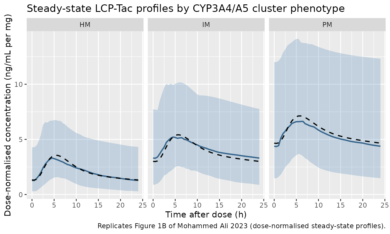
Replicates Figure 1B of Mohammed Ali 2023: dose-normalised steady-state whole-blood tacrolimus profiles after LCP-Tac, here stratified by CYP3A4/A5 cluster phenotype. Solid line = median, ribbon = 5th-95th percentile of the simulated cohort; dashed line = typical-value (zeroRe) prediction.
Absorption delay
The transit chain is the structural feature the paper emphasises: LCP-Tac shows a delayed, flattened absorption profile relative to immediate-release tacrolimus. The typical-value curves peak well after dosing, consistent with the reported mean transit time of 2.91 h.
typ |>
  group_by(cluster) |>
  slice_max(Cc, n = 1, with_ties = FALSE) |>
  ungroup() |>
  transmute(
    `Cluster phenotype` = cluster,
    `Typical Tmax (h)` = tad,
    `Typical Cmax (ng/mL per mg)` = round(Cc, 2)
  ) |>
  knitr::kable(
    caption = "Typical-value steady-state Tmax and Cmax per cluster phenotype (zeroRe simulation, 1 mg once daily)."
)| Cluster phenotype | Typical Tmax (h) | Typical Cmax (ng/mL per mg) |
|---|---|---|
| HM | 5.5 | 3.56 |
| IM | 5.5 | 5.41 |
| PM | 6.0 | 7.13 |
PKNCA validation
Steady-state NCA is computed over the final dosing interval using PKNCA. The cluster phenotype is the treatment grouping variable so the results can be compared directly against the per-phenotype exposures in Table 2.
sim_nca <- sim |>
  dplyr::filter(!is.na(Cc)) |>
  dplyr::select(id, time, Cc, cluster)

# Guarantee a time = 0 row per (id, cluster). LCP-Tac is an oral (extravascular)
# formulation, so the pre-first-dose concentration is 0.
sim_nca <- dplyr::bind_rows(
  sim_nca,
  sim_nca |> dplyr::distinct(id, cluster) |>
    dplyr::mutate(time = 0, Cc = 0)
) |>
  dplyr::distinct(id, cluster, time, .keep_all = TRUE) |>
  dplyr::arrange(id, cluster, time)

dose_df <- events |>
  dplyr::filter(evid == 1) |>
  dplyr::select(id, time, amt, cluster)

conc_obj <- PKNCA::PKNCAconc(sim_nca, Cc ~ time | cluster + id,
                             concu = "ng/mL", timeu = "h")
dose_obj <- PKNCA::PKNCAdose(dose_df, amt ~ time | cluster + id,
                             doseu = "mg")

intervals <- data.frame(
  start   = t_last,
  end     = t_last + tau,
  cmax    = TRUE,
  tmax    = TRUE,
  cmin    = TRUE,
  auclast = TRUE,
  cav     = TRUE
)

nca_res <- PKNCA::pk.nca(PKNCA::PKNCAdata(conc_obj, dose_obj, intervals = intervals))
Comparison against published exposure metrics
Table 2 of Mohammed Ali 2023 reports dose-normalised trough (C0/D)
and dose-normalised AUC (AUC/D) as geometric means per cluster
phenotype. Because the simulated dose is 1 mg, the simulated
AUC0-tau and Cmin are already on the
dose-normalised scale and are directly comparable. Cmin –
the lowest concentration over the dosing interval, which for this
delayed-absorption profile occurs at the pre-dose time point – is the
model analogue of the paper’s pre-dose trough C0 at steady state.
published <- tibble::tribble(
  ~cluster, ~auclast, ~cmin,
  "HM",     51,       1.23,
  "IM",     92,       2.91,
  "PM",     122,      4.04
)

cmp <- nlmixr2lib::ncaComparisonTable(
  simulated     = nca_res,
  reference     = published,
  by            = "cluster",
  units         = c(auclast = "ng*h/mL per mg", cmin = "ng/mL per mg"),
  tolerance_pct = 20
)

knitr::kable(
  cmp,
  caption = paste(
    "Simulated steady-state exposure (median of 200 virtual subjects per arm,",
    "1 mg once daily) versus the geometric-mean dose-normalised AUC and C0",
    "reported in Mohammed Ali 2023 Table 2.",
    "* differs from reference by >20%."
  ),
  align = c("l", "l", "r", "r", "r")
)| NCA parameter | cluster | Reference | Simulated | % diff |
|---|---|---|---|---|
| Cmin (ng/mL per mg) | HM | 1.23 | 1.26 | +2.7% |
| Cmin (ng/mL per mg) | IM | 2.91 | 3.29 | +13.2% |
| Cmin (ng/mL per mg) | PM | 4.04 | 4.35 | +7.7% |
| AUClast (ng*h/mL per mg) | HM | 51 | 49.3 | -3.4% |
| AUClast (ng*h/mL per mg) | IM | 92 | 98.4 | +7.0% |
| AUClast (ng*h/mL per mg) | PM | 122 | 127 | +4.5% |
Analytical cross-check of the clearance estimates
For a linear model at steady state,
AUC0-tau / Dose = 1 / (CL/F). This closed form lets the
packaged clearance estimates be checked against Table 2 without relying
on the simulation at all.
tibble::tibble(
  cluster = c("HM", "IM", "PM"),
  `CL/F (L/h), Table 3` = c(19.6, 10.6, 7.37)
) |>
  mutate(
    `Predicted AUC/D (ng*h/mL per mg)` = round(1000 / `CL/F (L/h), Table 3`, 1),
    `Published AUC/D (Table 2)` = c(51, 92, 122),
    `% difference` = round(
      100 * (`Predicted AUC/D (ng*h/mL per mg)` - `Published AUC/D (Table 2)`) /
        `Published AUC/D (Table 2)`, 1)
  ) |>
  dplyr::rename("Cluster phenotype" = cluster) |>
  knitr::kable(
    caption = paste(
      "Dose-normalised steady-state AUC implied by the Table 3 clearance",
      "estimates (1000 / (CL/F), converting mg/L to ng/mL) versus the",
      "geometric-mean AUC/D of Table 2."
    )
)| Cluster phenotype | CL/F (L/h), Table 3 | Predicted AUC/D (ng*h/mL per mg) | Published AUC/D (Table 2) | % difference |
|---|---|---|---|---|
| HM | 19.60 | 51.0 | 51 | 0.0 |
| IM | 10.60 | 94.3 | 92 | 2.5 |
| PM | 7.37 | 135.7 | 122 | 11.2 |
The high- and intermediate-metabolizer predictions agree with the
observed dose-normalised AUC to within ~3%. The poor-metabolizer
prediction is ~11% above the observed geometric mean, which is expected:
Table 2 reports only N = 2 AUC observations in the PM group
(95% CI 76-194 ng*h/mL per mg), so the observed PM geometric mean is
very imprecise, whereas the model’s CL/F PM estimate was
informed by all 46 PM trough observations as well.
Distribution of simulated exposures
auc_by_id <- as.data.frame(nca_res$result) |>
  filter(PPTESTCD == "auclast")

ggplot(auc_by_id, aes(cluster, PPORRES)) +
  geom_boxplot(outlier.alpha = 0.3, fill = "grey90") +
  geom_point(
    data = published,
    aes(cluster, auclast),
    colour = "firebrick", size = 3, shape = 18
  ) +
  scale_y_log10() +
  labs(
    x = "CYP3A4/A5 cluster phenotype",
    y = "Dose-normalised AUC0-tau (ng*h/mL per mg)",
    caption = "Red diamonds are the Table 2 geometric means of Mohammed Ali 2023."
  )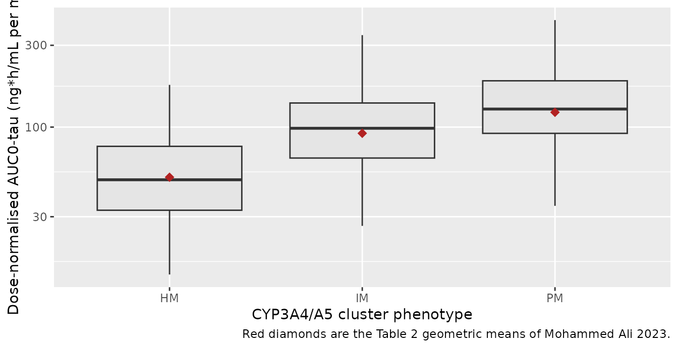
Simulated steady-state dose-normalised AUC0-tau by cluster phenotype (1 mg once daily, 200 virtual subjects per arm). Red diamonds are the geometric means reported in Mohammed Ali 2023 Table 2.
Assumptions and deviations
-
Transit-chain length. Mohammed Ali 2023 reports
NN = 2transit compartments fixed andMTT = 2.91 h, and cites Savic 2007 (reference [39]) as the method. The Savic parameterisation definesMTT = (n + 1) / ktr, so the packaged model usesktr = 3 / MTTand a chain of three first-order transfers from the dosing compartment into the absorption compartment. The paper does not print the transit equations or supply a NONMEM control stream, so this follows the cited method rather than a printed equation. Under the alternative reading (ktr = NN / MTT), the reported mean transit time would no longer be 2.91 h, which is why the Savic form was used. Compartmentstransit1andtransit2are the two Savic transit compartments proper;transit3is the Savic absorption compartment from whichKaoperates. -
Number of IOV occasions. Table 3 reports a single
IOV magnitude (44.8%) on
CL/Fbut does not state how many occasions were used. The packaged model provides five occasion slots (OCC = 1..5), the upper bound implied by Methods 2.1 (“from one to five C0 samples per patient were obtained”), with occasions 2-5 fixed to occasion 1’s variance (the NONMEM$OMEGA BLOCK(1) SAMEpattern). Records withOCCoutside 1-5 simply carry no IOV. The vignette simulates a single occasion (OCC = 1). -
IIV / IOV scale conversion. Table 3 gives
variability as CV percentages without stating whether they are
100 * sqrt(omega^2)or the exact log-normal100 * sqrt(exp(omega^2) - 1). The packaged model uses the exact log-normal relationomega^2 = log(CV^2 + 1), the nlmixr2lib convention. The two differ by under 10% (relative) at the largest reported CV (75%). -
Cluster-phenotype encoding. The paper’s three-level
cluster covariate is stored as its two underlying genotype columns
(
CYP3A5_EXPRandSNP_CYP3A4_RS35599367) and reassembled insidemodel(), per the convention documented ininst/references/covariate-columns.md. This keeps the underlying biology explicit and lets a downstream user re-derive a different clustering rule. Intermediate metabolizers arise from two different genotype combinations, which the model treats identically – exactly as Methods 2.3 defines them. The vignette’s IM arm uses the dominant combination (CYP3A5*3/*3,CYP3A4*22non-carrier). -
Covariates screened but not retained. Body weight,
BMI, age, sex, hematocrit and ABCB1 c.3435C>T were tested and
rejected (Results 3.2). They are documented in the model file’s
covariatesDataExcludedlist and are not referenced inmodel(). In particular the paper reports that allometric inclusion of body weight worsened the fit, so the packaged model carries no allometric scaling – unusual for an adult popPK model and deliberate here. -
Intermediate covariate models not packaged. The
paper also reports a CYP3A5-only covariate model (
CL/F20.4 L/h in expressers versus 10.1 L/h in nonexpressers) as a step in the covariate-building sequence. Only the final cluster model (Table 3) is packaged, per the base-versus-final policy. - Virtual cohort. All simulated subjects receive 1 mg once daily for 21 days (the poor-metabolizer arm, which has the longest terminal half-life at ~66 h, is then within ~1% of steady state). The real study population received 0.5-12 mg daily (median 2 mg); a single dose level is sufficient because the model is linear in dose and the paper’s Table 2 comparisons are dose-normalised.
-
No non-paper-derived parameter values. Every value
in
ini()comes from Table 3 or the Results text of Mohammed Ali 2023; nothing was digitised from a figure, obtained by correspondence, or carried from an upstream model.