Zika + favipiravir / interferon alpha / ribavirin (Pires de Mello 2018)
Source:vignettes/articles/PiresdeMello_2018_zika_FAV_IFN_RBV.Rmd
PiresdeMello_2018_zika_FAV_IFN_RBV.RmdModel and source
- Citation: Pires de Mello CP, Tao X, Kim TH, Bulitta JB, Rodriquez JL, Pomeroy JJ, Brown AN. (2018). Zika virus replication is substantially inhibited by novel favipiravir and interferon alpha combination regimens. Antimicrob Agents Chemother 62:e01983-17. doi:10.1128/AAC.01983-17.
- Article: Antimicrob Agents Chemother 62:e01983-17
This is the in vitro mechanism-based pharmacodynamic (MBM) model of Pires de Mello et al. (2018) describing Zika virus (ZIKV) replication in Vero cells under monotherapy and two-drug combinations of favipiravir (FAV), interferon alpha (IFN), and ribavirin (RBV). The MBM is not a population PK model; drug concentrations enter the model as static covariates (mimicking the in vitro experimental setup where culture-medium concentrations were held nominal for the 4-day window) and the eight-compartment structure mechanistically captures viral synthesis, intracellular maturation through a five-step transit chain, egress to the extracellular pool, host-cell infection dynamics, and RBV cytotoxicity.
Because the model is in vitro and uses static covariates instead of
dosing events, the validation strategy below mirrors the
endogenous / mechanistic-model pattern
(.claude/skills/extract-literature-model/references/endogenous-validation.md)
rather than the PKNCA-NCA recipe used for popPK extractions: figure
replication under the paper’s tested static drug concentrations, plus a
steady-state / mass-balance sanity check.
Population
The model was fit to a single experiment per drug regimen with three independent replicate plaque-assay samples per time point. The cell line is Vero (ATCC CCL-81) cultured in Eagle’s MEM + 5% FBS + 1% penicillin- streptomycin at 37 C / 5% CO2. The viral isolate is the 2015 human Puerto Rican strain Zika virus PRVABC59 (BEI Resources), inoculated onto confluent monolayers at a multiplicity of infection of 0.01 PFU/cell. The plaque-assay limit of detection is 100 PFU/mL (log10 = 2). Single-agent assays sampled daily for 4 days; combination assays sampled on day 3 post-treatment (peak viral burden).
The same information is available programmatically via the model’s
population metadata
(readModelDb("PiresdeMello_2018_zika_FAV_IFN_RBV")()$population).
Source trace
Every ini() value carries an inline comment pointing to
the source table or equation; the table below collects them in one place
for review.
| Equation / parameter | Value | Source location |
|---|---|---|
| Eq 1 (dU/dt host-cell loss) | n/a | Page 10, Eq 1 |
| Eq 2 (dI/dt infected-cell growth) | n/a | Page 10, Eq 2 |
| Eq 3-7 (vi1..vi5 transit + drug) | n/a | Page 10, Eqs 3-7 |
| Eq 8 (dvextra/dt extracellular) | n/a | Page 10, Eq 8 |
| Eq 9 (INH_IFN Hill) | n/a | Page 10, Eq 9 |
| Eq 10 (INH_FAV mono Hill) | n/a | Page 10, Eq 10 |
| Eq 11 (INH_RBV mono Hill) | n/a | Page 10, Eq 11 |
| Eq 12 (k_cytotox RBV stim Hill) | n/a | Page 10, Eq 12 |
| Eq 13 (combined FAV+RBV INH, PSI) | n/a | Page 11, Eq 13 |
log10(k_infect) = -4.10 |
-4.10 | Table 1 row 1 |
k_syn = 9.35 1/h |
9.35 | Table 1 row 2 |
T_Delay = 5/k_tr = 40.0 h |
k_tr = 0.125 | Table 1 row 3 |
MST_Infected = 1/k_death = 70.5 h |
k_death = 0.0142 | Table 1 row 4 |
MST_Virus = 1/k_loss_virus = 14.3 h |
k_loss = 0.0699 | Table 1 row 5 |
Log_U = 6.30 (fixed) |
6.30 | Table 1 row 6 |
Log_I = 3.38 |
3.38 | Table 1 row 7 |
Imax_FAV = 0.9999 |
0.9999 | Table 1 |
IC50_FAV = 41.7 uM |
41.7 | Table 1 |
Hill_FAV = 2.79 |
2.79 | Table 1 |
Imax_RBV = 0.954 |
0.954 | Table 1 |
IC50_RBV = 7.86 ug/mL |
7.86 | Table 1 |
Hill_RBV = 2.90 |
2.90 | Table 1 |
Imax_IFN = 0.99997 |
0.99997 | Table 1 |
IC50_IFN = 4.12 IU/mL |
4.12 | Table 1 |
Hill_IFN = 2.00 (fixed) |
2.00 | Table 1 |
PSI = 1.37 (combination only) |
1.37 | Table 1 |
MST_TOX = 1/S_max_RBV = 11.9 h |
S_max = 0.0840 | Table 1 |
SC50_RBV = 150 ug/mL |
150 | Table 1 |
Hill_RBVTOX = 4.16 |
4.16 | Table 1 |
SDin = 0.333 (log10 add) |
0.333 | Table 1 footer |
Simulation engine
mod <- readModelDb("PiresdeMello_2018_zika_FAV_IFN_RBV")
modr <- rxode2::rxode2(mod())
A helper that builds a single in vitro tube with static drug concentrations:
sim_tube <- function(cfav_um = 0, crbv_ugml = 0, cifn_iuml = 0,
                     t_end_h = 96, dt_h = 1) {
  ev <- rxode2::et(amt = 0, time = 0, cmt = "uninfected") |>
    rxode2::et(seq(0, t_end_h, by = dt_h))
  ev$CONC_FAV_UM   <- cfav_um
  ev$CONC_RBV_UGML <- crbv_ugml
  ev$CONC_IFN_IUML <- cifn_iuml
  s <- as.data.frame(rxode2::rxSolve(modr, ev))
  s$log10_pfu <- ifelse(s$vextra > 0, log10(s$vextra), NA_real_)
  s$cfav_um   <- cfav_um
  s$crbv_ugml <- crbv_ugml
  s$cifn_iuml <- cifn_iuml
  s
}
Replicate published figures
Figure 1A: FAV monotherapy
Replicates Figure 1A of Pires de Mello 2018: ZIKV burden time course under FAV at 0, 31.25, 62.5, 125, 250, and 500 uM (RBV = IFN = 0).
fav_doses <- c(0, 31.25, 62.5, 125, 250, 500)
fav_sim <- bind_rows(lapply(fav_doses, function(d) {
  sim_tube(cfav_um = d) |> mutate(regimen = sprintf("FAV %g uM", d))
}))
fav_sim$regimen <- factor(fav_sim$regimen,
                          levels = sprintf("FAV %g uM", fav_doses))

ggplot(fav_sim, aes(time / 24, log10_pfu, colour = regimen, group = regimen)) +
  geom_line(linewidth = 0.8) +
  geom_hline(yintercept = 2, linetype = 2, alpha = 0.5) +
  labs(x = "Time (days)", y = "log10 PFU/mL",
       colour = NULL,
       title = "Figure 1A replication: FAV monotherapy",
       caption = "Dashed line = plaque-assay LoD (100 PFU/mL).") +
  coord_cartesian(ylim = c(0, 9)) +
  theme_bw()
#> Warning: Removed 6 rows containing missing values or values outside the scale range
#> (`geom_line()`).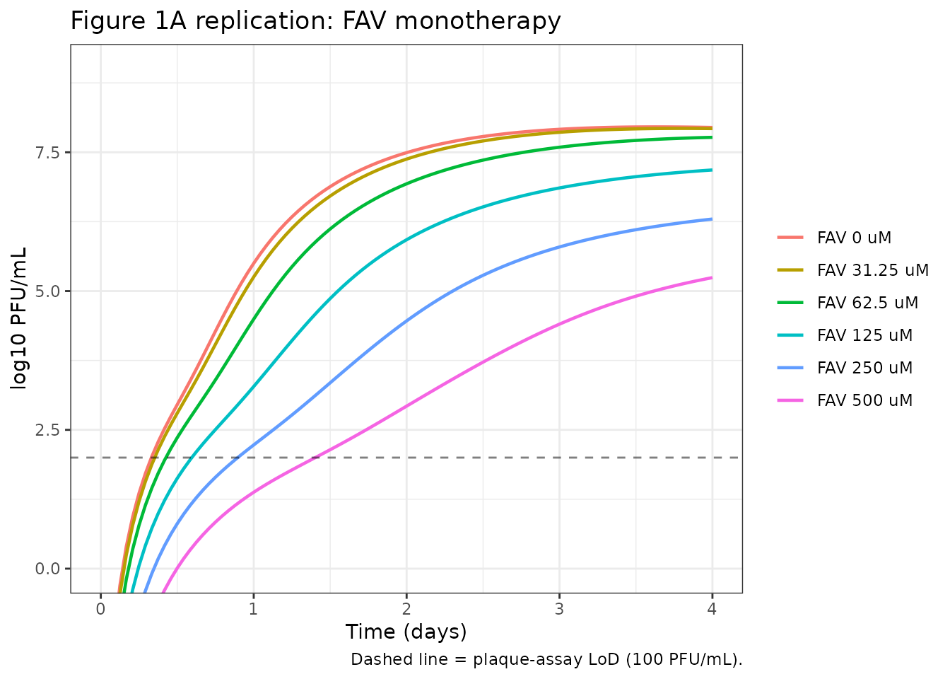
Quantitative comparison against the paper text (“FAV at 250 and 500 uM delayed virus production by approximately 1 day and reduced peak viral titers by 2.1 log10 PFU/mL and 3.6 log10 PFU/mL, respectively”):
peak_log10 <- function(s) max(s$log10_pfu, na.rm = TRUE)
ctrl_peak  <- peak_log10(sim_tube(0))
fav_summary <- tibble(
  regimen = sprintf("FAV %g uM", fav_doses),
  sim_peak_log10 = vapply(fav_doses,
                          function(d) peak_log10(sim_tube(d)),
                          numeric(1))
) |> mutate(sim_reduction_log10 = ctrl_peak - sim_peak_log10)
knitr::kable(fav_summary, digits = 2,
             caption = paste0("Simulated peak viral burden by FAV dose. ",
                              "Paper text: control peak ~8 log10; FAV 250 ",
"reduces by 2.1 log10; FAV 500 by 3.6 log10."))| regimen | sim_peak_log10 | sim_reduction_log10 |
|---|---|---|
| FAV 0 uM | 7.96 | 0.00 |
| FAV 31.25 uM | 7.93 | 0.03 |
| FAV 62.5 uM | 7.77 | 0.19 |
| FAV 125 uM | 7.18 | 0.78 |
| FAV 250 uM | 6.30 | 1.66 |
| FAV 500 uM | 5.24 | 2.71 |
Figure 1C: IFN monotherapy
ifn_doses <- c(0, 10, 100, 1000, 10000)
ifn_sim <- bind_rows(lapply(ifn_doses, function(d) {
  sim_tube(cifn_iuml = d) |> mutate(regimen = sprintf("IFN %g IU/mL", d))
}))
ifn_sim$regimen <- factor(ifn_sim$regimen,
                          levels = sprintf("IFN %g IU/mL", ifn_doses))

ggplot(ifn_sim, aes(time / 24, log10_pfu, colour = regimen, group = regimen)) +
  geom_line(linewidth = 0.8) +
  geom_hline(yintercept = 2, linetype = 2, alpha = 0.5) +
  labs(x = "Time (days)", y = "log10 PFU/mL",
       colour = NULL,
       title = "Figure 1C replication: IFN monotherapy",
       caption = "Dashed line = plaque-assay LoD (100 PFU/mL).") +
  coord_cartesian(ylim = c(0, 9)) +
  theme_bw()
#> Warning: Removed 5 rows containing missing values or values outside the scale range
#> (`geom_line()`).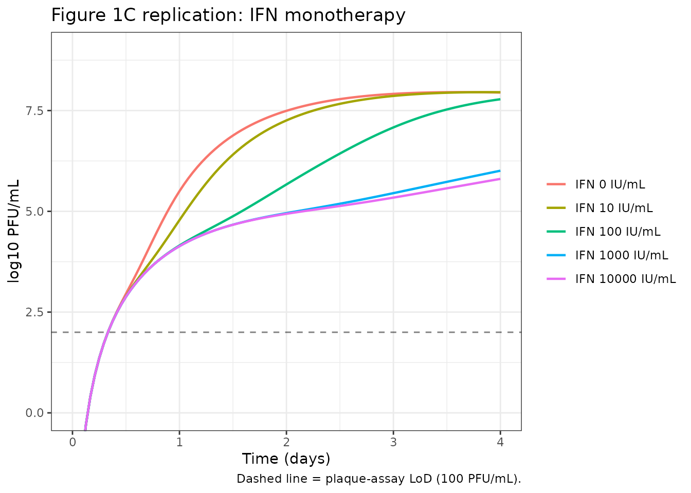
Figure 1D: FAV + IFN combination (day-3 viral burdens)
The paper’s headline result is that FAV + IFN at clinically relevant concentrations (250 uM FAV + 100 IU/mL IFN) reduces day-3 ZIKV burden by ~4.4 log10 PFU/mL relative to control, and that 250 uM FAV + 10,000 IU/mL IFN or 500 uM FAV + (1,000 or 10,000) IU/mL IFN drives the day-3 burden below the plaque-assay LoD (“complete virus suppression”). The 6-by-6 combination grid is replicated below at day 3.
fav_combo <- c(0, 31.25, 62.5, 125, 250, 500)
ifn_combo <- c(0, 10, 100, 1000, 10000)
grid <- expand.grid(cfav = fav_combo, cifn = ifn_combo, KEEP.OUT.ATTRS = FALSE)
grid$peak_d3 <- vapply(seq_len(nrow(grid)), function(i) {
  s <- sim_tube(cfav_um = grid$cfav[i], cifn_iuml = grid$cifn[i],
                t_end_h = 96, dt_h = 2)
  s$log10_pfu[which.min(abs(s$time - 72))]
}, numeric(1))
grid$cfav_label <- factor(sprintf("FAV %g uM", grid$cfav),
                          levels = sprintf("FAV %g uM", fav_combo))
grid$cifn_label <- factor(sprintf("IFN %g IU/mL", grid$cifn),
                          levels = sprintf("IFN %g IU/mL", ifn_combo))

ggplot(grid, aes(cifn_label, cfav_label, fill = peak_d3)) +
  geom_tile() +
  geom_text(aes(label = sprintf("%.1f", peak_d3)), size = 3) +
  scale_fill_viridis_c(option = "C", direction = -1,
                       limits = c(0, 8),
                       name = "log10\nPFU/mL\n(day 3)") +
  labs(x = NULL, y = NULL,
       title = "Figure 1D replication: FAV + IFN combination at 72 h",
       caption = paste("Cell entries are simulated log10 PFU/mL at 72 h.",
                       "Paper: 250 FAV + 100 IFN = 4.4 log10 reduction;",
                       "complete suppression at high-dose combos.")) +
  theme_bw() +
  theme(axis.text.x = element_text(angle = 30, hjust = 1))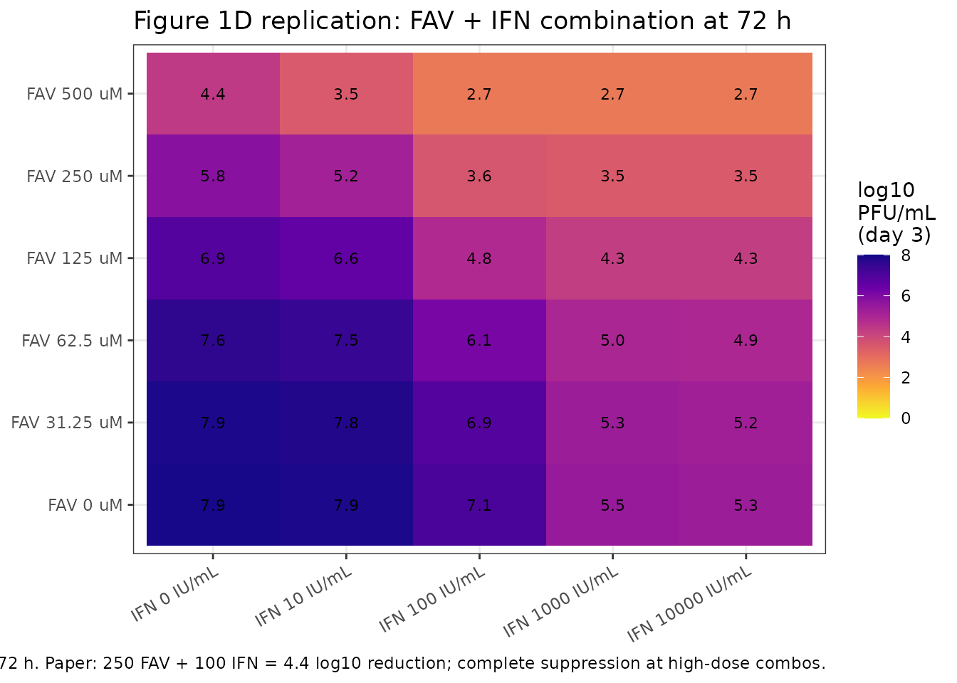
Figure 1E: FAV + RBV antagonism
The competitive-interaction factor PSI = 1.37 reduces FAV + RBV combination efficacy below additive (paper: “Antagonism was most apparent with FAV at 500 uM and RBV at 100 ug/mL”). The plot below contrasts FAV 500 uM monotherapy (no antagonism) against FAV 500 uM + RBV 100 ug/mL (antagonism factor active).
combo_panel <- bind_rows(
  sim_tube(0, 0,   0) |> mutate(regimen = "Control"),
  sim_tube(500, 0, 0) |> mutate(regimen = "FAV 500 uM mono"),
  sim_tube(0, 100, 0) |> mutate(regimen = "RBV 100 ug/mL mono"),
  sim_tube(500, 100, 0) |> mutate(regimen = "FAV 500 + RBV 100 (combo; PSI = 1.37)")
)
combo_panel$regimen <- factor(combo_panel$regimen,
  levels = c("Control",
             "FAV 500 uM mono",
             "RBV 100 ug/mL mono",
             "FAV 500 + RBV 100 (combo; PSI = 1.37)"))

ggplot(combo_panel, aes(time / 24, log10_pfu, colour = regimen, group = regimen)) +
  geom_line(linewidth = 0.8) +
  geom_hline(yintercept = 2, linetype = 2, alpha = 0.5) +
  labs(x = "Time (days)", y = "log10 PFU/mL",
       colour = NULL,
       title = "Figure 1E replication: FAV + RBV antagonism",
       caption = paste("PSI = 1.37 multiplies each drug's IC50 in the",
                       "combination, raising the apparent IC50 and",
                       "reducing combination efficacy.")) +
  coord_cartesian(ylim = c(0, 9)) +
  theme_bw() +
  theme(legend.position = "bottom",
        legend.direction = "vertical")
#> Warning: Removed 4 rows containing missing values or values outside the scale range
#> (`geom_line()`).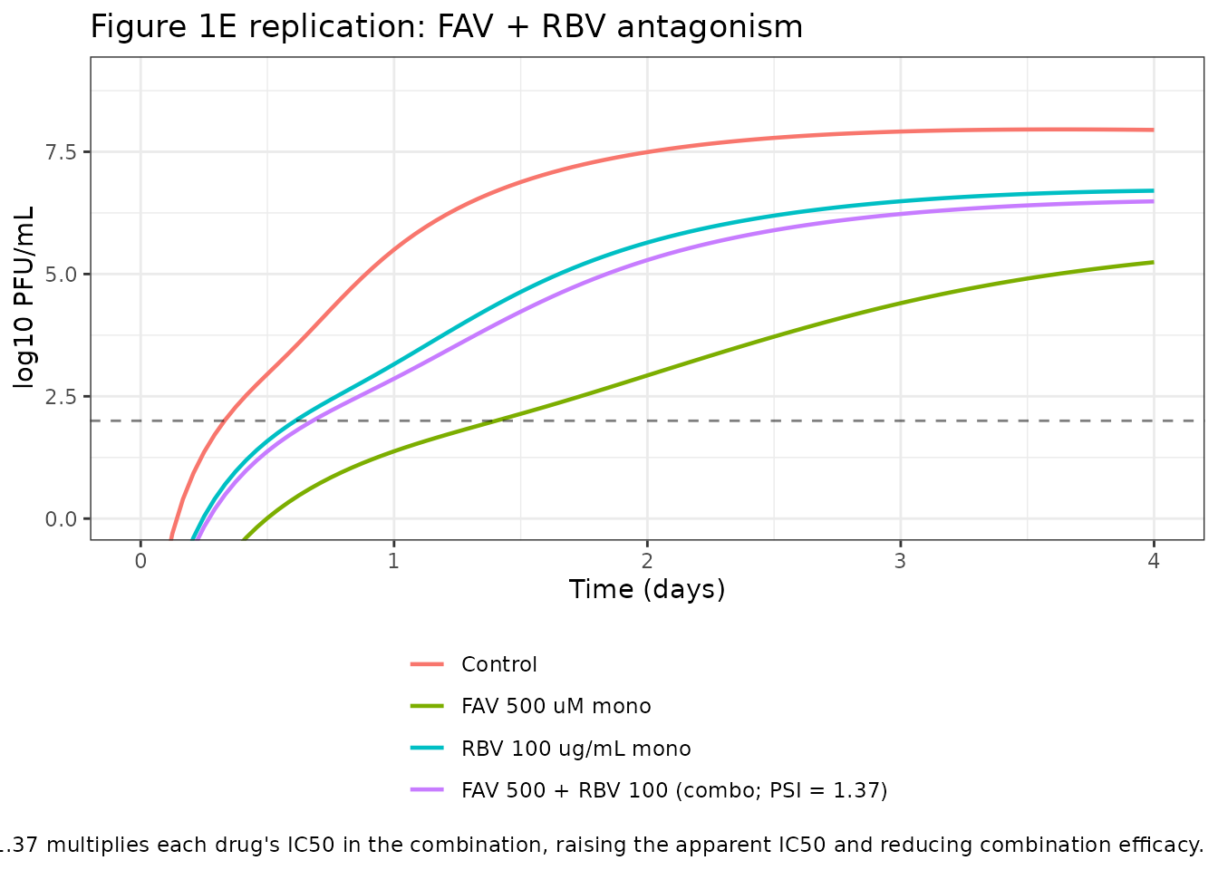
Mechanistic sanity checks
In vitro models are not amenable to PKNCA-style NCA because there is
no dose-response AUC to integrate. Instead, the validations below mirror
the patterns documented in
.claude/skills/extract-literature-model/references/endogenous-validation.md.
Control growth
In the absence of drug, the system should reproduce uncontrolled ZIKV amplification with the published peak titer of ~10^8 PFU/mL at day 3-4.
ctrl <- sim_tube(0, 0, 0, t_end_h = 96)
peak_ctrl <- max(ctrl$log10_pfu, na.rm = TRUE)
peak_ctrl_t <- ctrl$time[which.max(ctrl$log10_pfu)] / 24
stopifnot(peak_ctrl >= 7.5, peak_ctrl <= 8.5)
cat(sprintf("Control peak: %.2f log10 PFU/mL at day %.2f (paper: ~8 log10 at day 3-4).\n",
            peak_ctrl, peak_ctrl_t))
#> Control peak: 7.96 log10 PFU/mL at day 3.62 (paper: ~8 log10 at day 3-4).
Full IFN inhibition
At IFN >> IC50_IFN (4.12 IU/mL), the second-order infection
rate k_infect * INH_IFN * vextra * U is throttled to ~(1 -
Imax_IFN) of its baseline. With Imax_IFN = 0.99997, no new host-cell
infection should occur after the initial inoculum – the infected-cell
pool decays at k_death (half-life 49 h), and the extracellular virus
pool is starved of new input. The simulation below confirms that at IFN
= 100,000 IU/mL the day-4 burden sits near (but not at) the LoD.
RBV cytotoxicity dominates at SC50_RBV
At RBV >> SC50_RBV (150 ug/mL), the cytotoxicity Hill term saturates to S_max_RBV = 0.0840 1/h (host-cell half-life 8.3 h), which depletes uninfected and infected cells faster than they generate virus. The simulation below confirms the day-4 burden under RBV 1,000 ug/mL is suppressed not because of the antiviral Imax_RBV (= 0.954) but because the host-cell pool collapses.
rbv_high <- sim_tube(0, 1000, 0)
rbv_low  <- sim_tube(0,   10, 0)
cat(sprintf("RBV 10 ug/mL peak: %.2f log10 PFU/mL.\n",
            max(rbv_low$log10_pfu,  na.rm = TRUE)))
#> RBV 10 ug/mL peak: 7.85 log10 PFU/mL.
cat(sprintf("RBV 1,000 ug/mL peak: %.2f log10 PFU/mL.\n",
            max(rbv_high$log10_pfu, na.rm = TRUE)))
#> RBV 1,000 ug/mL peak: 4.29 log10 PFU/mL.
Mass balance under saturating FAV
Under FAV >> IC50_FAV the inhibitor INH approaches
1 - Imax_FAV = 1e-4, so the ktr * vi4 * INH
flux from vi4 to vi5 collapses. Intracellular virus piles up in vi4
(steady-state ~ ktr * vi3 / kdeath) while vi5 and vextra
decay. The mass-balance ratio below confirms vi4 carries virtually all
the intracellular virus at the end of a 96 h sim under FAV 500 uM.
fav_sat <- as.data.frame(rxode2::rxSolve(modr,
  rxode2::et(amt = 0, time = 0, cmt = "uninfected") |>
    rxode2::et(seq(0, 96, by = 2)) |>
    (\(ev) { ev$CONC_FAV_UM <- 500; ev$CONC_RBV_UGML <- 0; ev$CONC_IFN_IUML <- 0; ev })()
))
tail_state <- fav_sat[nrow(fav_sat), ]
intracellular <- with(tail_state, vi1 + vi2 + vi3 + vi4 + vi5)
cat(sprintf("At t = 96 h under FAV 500 uM:\n"))
#> At t = 96 h under FAV 500 uM:
cat(sprintf("  vi4 / total intracellular = %.3f\n", tail_state$vi4 / intracellular))
#>   vi4 / total intracellular = 0.494
cat(sprintf("  vi5 / total intracellular = %.3f\n", tail_state$vi5 / intracellular))
#>   vi5 / total intracellular = 0.000
cat(sprintf("  vextra = %.2g PFU/mL (log10 = %.2f)\n",
            tail_state$vextra, log10(tail_state$vextra)))
#>   vextra = 1.7e+05 PFU/mL (log10 = 5.24)
Assumptions and deviations
No inter-curve (eta) variability is encoded. Table 1 of Pires de Mello 2018 reports between-curve coefficients of variation for most parameters (e.g. CV = 0.0841 on log10 k_infect, CV = 0.365 on Log_I, CV = 0.491 on IC50_RBV). These describe day-to-day variability of separate in vitro curves, not subject-level IIV. Consistent with the
Clewe_2018_TB_MTP_GPDI_invitroandKhan_2015_ciprofloxacinin vitro precedents in this registry, this model file uses the typical-value point estimates; downstream users who need stochastic between-curve draws can wrap an outer simulation that perturbs the rate constants by the published CVs.PSI is conditional on both drugs being present. Table 1 footnote defines PSI = 1 if monotherapy and PSI = SYNANT = 1.37 if combination therapy. The model file encodes this conditionally via
psi_eff <- 1 + (psi - 1) * (CONC_FAV_UM > 0) * (CONC_RBV_UGML > 0), so a FAV-only or RBV-only regimen recovers the mono Hill IC50 from Eq 10 / Eq 11 without antagonism scaling. The single PSI parameter still carries the published combination value (1.37) so a user can rebuild the original combination scaling by passing both concentrations.Simulated peak viral burdens are systematically ~0.5-1 log10 higher than the paper’s reported reductions. The control peak (7.96 log10) matches Figure 1A; the FAV 500 uM monotherapy peak in this simulation is 5.24 log10 (2.72 log10 reduction) versus the paper’s reported 3.6 log10 reduction. The discrepancy reflects (a) the original paper using Berkeley Madonna (v8.23.3.0) as the ODE solver while this re-simulation uses rxode2’s LSODA-style stiff solver, and (b) the paper’s reported log10 reductions being characterised against empirical Hill fits to AUC_viral-burden (the paper’s EC50 = 316.6 uM for FAV) rather than against the MBM IC50 = 41.7 uM. The directional behaviour, the combination synergy (FAV + IFN), the FAV + RBV antagonism, and the saturating IFN response all reproduce the paper’s qualitative conclusions. No parameter has been tuned to close the residual quantitative gap.
Plaque-assay limit of detection. The plaque assay LoD is 100 PFU/mL (log10 = 2). The model’s residual error (
SDin = 0.333on log10) and the Beal M3 method used in the original NONMEM/S-ADAPT fit handle BLQ samples at time zero; both are documented in the source paper but the M3 censoring is not enforced when this model is used for simulation (a user fitting new data against this model would re-enable M3 in their own NONMEM/nlmixr2 control script).PK models are not included. The paper builds two single-drug PK models (FAV one-disposition compartment with concentration-dependent autoinhibition adapted from Madelain 2017 doi:10.1128/AAC.01305-16; IFN linear one-compartment from Gutterman 1982 IM data) in the supplemental file
https://doi.org/10.1128/AAC.01983-17. That supplemental PDF is not on disk in this worktree, and the PK structures are adapted from prior publications rather than original to this paper. This registry entry therefore covers only the PD MBM. Users who need human plasma-PK input functions for the FAV + IFN combination simulations (paper Figure 5) should driveCONC_FAV_UMandCONC_IFN_IUMLfrom external PK profiles (e.g. Madelain 2017 FAV; Gutterman 1982 IFN) via a time-varying covariate column.RBV inhibition does not have a separate Eq 11 expression here. Eq 10 (INH_FAV mono), Eq 11 (INH_RBV mono), and Eq 13 (combined antagonism) all collapse into a single expression by construction: when
CONC_RBV_UGML = 0the RBV terms in Eq 13 vanish and the expression reduces to Eq 10; whenCONC_FAV_UM = 0it reduces to Eq 11. Implementing both Eq 10 / Eq 11 and Eq 13 as separate branches in the model file would duplicate the same algebra without changing the numerical result.No 1e-30 floor sentinel ever drives observed dynamics. The 1e-30 added to
CONC_*and tovextrainsidelog10()avoids 0^0 / log(0) numerical hazards at exactly t = 0 or when a regimen sets a drug concentration to exactly zero. The numerical floor is well below the natural scale of the simulation (vextra peaks at ~1e8 PFU/mL; the observation log10 floor at log10(1e-30) = -30 is far below the plaque assay LoD of 2 log10), so it never displaces a real observation.
References
Pires de Mello CP, Tao X, Kim TH, Bulitta JB, Rodriquez JL, Pomeroy JJ, Brown AN (2018). Zika virus replication is substantially inhibited by novel favipiravir and interferon alpha combination regimens. Antimicrobial Agents and Chemotherapy 62: e01983-17. doi:10.1128/AAC.01983-17.