Remdesivir and GS-441524 (Leegwater 2022)
Source:vignettes/articles/Leegwater_2022_remdesivir.Rmd
Leegwater_2022_remdesivir.RmdModel and source
- Citation: Leegwater E, Moes DJAR, Bosma LBE, Ottens TH, van der Meer IM, van Nieuwkoop C, Wilms EB. Population Pharmacokinetics of Remdesivir and GS-441524 in Hospitalized COVID-19 Patients. Antimicrob Agents Chemother. 2022;66(6):e00254-22. doi:10.1128/aac.00254-22. Final estimates from Table 2; the compartment structure, the 0.1 x metabolic-clearance renal arm, the eGFR power term, the OMEGA variances and the additive residual-error form from the NONMEM control stream in Supplement 2 (‘FINAL model RDV+ GS-441524’, ADVAN5 TRANS1).
- Description: Integrated parent-metabolite population PK model for intravenous remdesivir and its circulating nucleoside metabolite GS-441524 in non-critically ill hospitalized adults with COVID-19 and hypoxemia (Leegwater 2022). One compartment for each analyte, coupled in series (NONMEM ADVAN5). The estimated remdesivir clearance is the metabolic arm that forms GS-441524; renal excretion of unchanged remdesivir is fixed at 10% of that metabolic clearance, so total remdesivir clearance is 1.1 times the metabolic clearance and the two arms share one random effect. BSA-normalized eGFR (CKD-EPI) enters GS-441524 clearance as a power function referenced to 94 mL/min/1.73 m^2. The parent-to-metabolite transfer is mass for mass with no molecular-weight correction, as in the source control stream, so the GS-441524 volume and clearance are apparent values that absorb the molar-mass ratio and any unformed fraction. Residual error is additive on the linear concentration scale for each analyte.
- Article: https://doi.org/10.1128/aac.00254-22 (open access, PMC9211420)
- Supplement (goodness-of-fit plots, pcVPCs, the final NONMEM control stream and the individual concentrations): available from the article page.
Leegwater et al. sampled 17 hospitalized COVID-19 patients six times on the first day of remdesivir therapy and fitted an integrated parent-metabolite model to remdesivir and GS-441524 plasma concentrations. They then used Monte Carlo simulation to compare four dosing regimens and three renal-function levels by the probability of reaching the in vitro EC50 of each analyte.
Population
Seventeen adults (one woman, 5.9%) hospitalized on the general ward of the Haga Teaching Hospital, The Hague, between January and July 2021 with RT-PCR-confirmed COVID-19 and a need for supplemental oxygen; all scored 5 on the WHO ordinal scale and all received dexamethasone (Table 1). Median age was 55 years (range 31-74), median body weight 92 kg (65-122), median BMI 30.9 kg/m^2 and median CKD-EPI eGFR 94 mL/min/1.73 m^2 (8-119). Thirty-five percent had diabetes mellitus and 29% cardiovascular disease. Patients received the licensed regimen: 200 mg intravenously on day 1 followed by 100 mg daily, each infused over 1 to 2 h. Six samples were scheduled 0.5, 1.5, 2.5, 6, 12 and 23 h after the end of the first infusion; 84 samples were obtained.
The same information is available programmatically via
readModelDb("Leegwater_2022_remdesivir")()$population.
Source trace
The per-parameter origin is recorded as an in-file comment next to
each ini() entry in
inst/modeldb/specificDrugs/Leegwater_2022_remdesivir.R. The
table below collects them. “S2” is the NONMEM control stream printed in
Supplement 2.
| Equation / parameter | Value | Source location |
|---|---|---|
lcl_met (remdesivir metabolic CL) |
log(207) L/h | Table 2 ‘Metabolic CL’; S2 $THETA(1),
CLtoM = TVCL*EXP(ETA(1))
|
lvc (remdesivir V) |
log(157) L | Table 2; S2 $THETA(2)
|
clrat_gs441524 (metabolic / renal CL) |
10, fixed | S2 CL = 0.1 * CLtoM; Table 2 ‘Renal CL 20.7 fixed’ |
lcl_gs441524 (GS-441524 CL at eGFR 94) |
log(27.6) L/h | Table 2; S2 $THETA(3)
|
lvc_gs441524 (GS-441524 V) |
log(1060) L | Table 2; S2 $THETA(4)
|
e_crcl_cl_gs441524 |
1.76 | Table 2 ‘eGFR on CL’; S2 $THETA(7),
(GFR/94)**THETA(7)
|
etalcl_met |
0.151 | S2 $OMEGA(1); Table 2 38.9% = sqrt(0.151) |
etalvc |
0.229 | S2 $OMEGA(2); Table 2 47.9% = sqrt(0.229) |
etalcl_gs441524 |
0.225 | S2 $OMEGA(3); Table 2 47.4% = sqrt(0.225) |
etalvc_gs441524 |
0.184 | S2 $OMEGA(4); Table 2 42.9% = sqrt(0.184) |
addSd (remdesivir) |
0.0294 mg/L | Table 2; S2 $THETA(5),
Y = IPRED + W*EPS(1), $SIGMA 1 FIX
|
addSd_gs441524 |
0.0140 mg/L | Table 2; S2 $THETA(6)
|
d/dt(central), d/dt(central_gs441524)
|
n/a | S2 $SUBROUTINES ADVAN5 TRANS1,
K10 = CL/V1, K12 = CLtoM/V1,
K20 = CLm/V2
|
Cc, Cc_gs441524
|
n/a | S2 $ERROR, IPRED = A(1)/V1 and
A(2)/V2
|
Structural checks against the reported half-lives
The paper reports an average elimination half-life of about 0.48 h for remdesivir and 26.6 h for GS-441524 (Results, ‘Pharmacokinetics’). With the renal arm at one tenth of the metabolic arm, total remdesivir clearance is 1.1 x 207 = 227.7 L/h; the closed-form half-lives from the typical values reproduce both numbers, which confirms that the 10% renal arm is added to, not carved out of, the 207 L/h.
mod <- readModelDb("Leegwater_2022_remdesivir")
ini_val <- function(name) {
  df <- rxode2::rxode(mod)$iniDf
  df$est[df$name == name]
}
cl_met <- exp(ini_val("lcl_met"))
#> ℹ parameter labels from comments will be replaced by 'label()'
cl_tot <- cl_met * (1 + 1 / ini_val("clrat_gs441524"))
#> ℹ parameter labels from comments will be replaced by 'label()'
t12_rdv <- log(2) * exp(ini_val("lvc")) / cl_tot
#> ℹ parameter labels from comments will be replaced by 'label()'
t12_gs <- log(2) * exp(ini_val("lvc_gs441524")) / exp(ini_val("lcl_gs441524"))
#> ℹ parameter labels from comments will be replaced by 'label()'
#> ℹ parameter labels from comments will be replaced by 'label()'
tibble(
  Quantity = c("Remdesivir renal CL (L/h)", "Remdesivir total CL (L/h)",
               "Remdesivir t1/2 (h)", "GS-441524 t1/2 (h)"),
  Model = signif(c(cl_met / ini_val("clrat_gs441524"), cl_tot, t12_rdv, t12_gs), 4),
  Paper = c(20.7, NA, 0.48, 26.6)
) |>
  knitr::kable(caption = "Typical-value clearance and half-lives.")
#> ℹ parameter labels from comments will be replaced by 'label()'| Quantity | Model | Paper |
|---|---|---|
| Remdesivir renal CL (L/h) | 20.7000 | 20.70 |
| Remdesivir total CL (L/h) | 227.7000 | NA |
| Remdesivir t1/2 (h) | 0.4779 | 0.48 |
| GS-441524 t1/2 (h) | 26.6200 | 26.60 |
Typical first-dose profile
The paper reports that GS-441524 reached its maximum 3.7 h after the start of treatment, averaging 173 ug/L during the first 24 h (Results, ‘Pharmacokinetics’). Infusion length in the study was 1 to 2 h and is not stated for the simulations, so the typical-value profile is solved for 1, 1.5 and 2 h infusions. The reported 3.7 h sits inside the bracket the three durations span.
make_events <- function(id, dose_times, doses, dur, crcl, obs_times) {
  dosing <- data.frame(
    id = id, time = dose_times, amt = doses, dur = dur, evid = 1L,
    cmt = "central", dvid = NA_integer_
  )
  obs <- data.frame(
    id = id, time = obs_times, amt = 0, dur = 0, evid = 0L,
    cmt = "central", dvid = 1L
  )
  dplyr::bind_rows(dosing, obs) |>
    dplyr::mutate(CRCL = crcl) |>
    dplyr::arrange(id, time, dplyr::desc(evid))
}

typ <- lapply(c(1, 1.5, 2), function(d) {
  ev <- make_events(1L, 0, 200, d, 94, seq(0, 24, by = 0.01))
  s <- as.data.frame(rxode2::rxSolve(mod, ev, omega = NA, sigma = NA))
  tibble(
    infusion_h = d,
    rdv_cmax_ugL = 1000 * max(s$Cc),
    gs_cmax_ugL = 1000 * max(s$Cc_gs441524),
    gs_tmax_h = s$time[which.max(s$Cc_gs441524)]
  )
}) |>
  dplyr::bind_rows()
#> ℹ parameter labels from comments will be replaced by 'label()'

typ |>
  dplyr::rename(
    "Infusion (h)" = infusion_h,
    "Remdesivir Cmax (ug/L)" = rdv_cmax_ugL,
    "GS-441524 Cmax (ug/L)" = gs_cmax_ugL,
    "GS-441524 Tmax (h)" = gs_tmax_h
  ) |>
knitr::kable(digits = 2, caption = "Typical patient (eGFR 94), 200 mg first dose.")| Infusion (h) | Remdesivir Cmax (ug/L) | GS-441524 Cmax (ug/L) | GS-441524 Tmax (h) |
|---|---|---|---|
| 1.0 | 672.38 | 159.13 | 3.38 |
| 1.5 | 519.07 | 158.83 | 3.71 |
| 2.0 | 415.02 | 158.44 | 4.05 |
Virtual cohort and first-day VPC against the published concentrations
Supplement 3 lists every measured concentration (time after the start of the first dose, mg/L; ‘BLD’ = below the limit of detection). The VPC below simulates 200 virtual patients receiving 200 mg over 1.5 h, with eGFR sampled from the cohort’s median and range (log-normal around 94 mL/min/1.73 m^2, truncated to 8-119), and overlays the observations.
obs_txt <- "
id time rdv gs
1 2.0 0.387 0.241
1 2.8 0.141 0.295
1 4.4 0.042 0.382
1 5.4 0.02 0.39
1 15.8 NA 0.53
1 20.0 NA 0.558
2 1.8 0.249 0.136
3 3.1 0.045 0.097
3 7.0 0.00185 0.091
3 9.1 NA 0.090
3 23.9 NA 0.055
4 1.8 0.246 0.105
4 2.8 0.05 0.111
4 4.1 0.021 0.124
4 8.0 0.0054 0.117
4 10.0 NA 0.108
4 24.7 NA 0.067
5 2.4 0.04 0.118
5 3.7 0.013 0.123
5 6.1 0.0034 0.125
5 20.7 NA 0.096
5 24.0 NA 0.084
6 2.3 0.052 0.114
6 3.3 0.018 0.128
6 4.2 0.0095 0.126
6 6.1 0.0024 0.118
6 17.2 NA 0.094
7 2.1 0.078 0.13
7 3.4 0.022 0.127
7 4.4 0.01 0.116
7 6.2 0.0052 0.108
7 17.3 NA 0.073
7 20.6 NA 0.061
8 1.8 0.171 0.14
8 2.8 0.044 0.157
8 3.8 0.023 0.163
8 4.8 0.011 0.175
8 15.2 NA 0.157
8 19.4 NA 0.119
9 2.0 0.261 0.127
9 3.0 0.069 0.115
9 4.3 0.022 0.107
10 2.1 0.118 0.126
10 3.0 0.029 0.12
10 3.9 0.012 0.109
11 2.1 0.128 0.191
11 2.8 0.041 0.186
11 3.7 0.023 0.189
11 7.2 0.0016 0.158
11 16.4 NA 0.16
11 22.9 NA 0.12
12 1.9 0.227 0.156
12 2.6 0.098 0.171
12 3.5 0.04 0.186
12 6.7 0.011 0.169
12 16.3 NA 0.178
12 22.4 NA 0.124
13 2.7 0.595 0.119
13 3.6 0.224 0.16
13 4.6 0.017 0.17
13 8.1 0.0023 0.161
13 17.1 NA 0.137
15 1.9 0.303 0.115
15 3.0 0.06 0.146
15 4.2 0.036 0.155
15 4.9 0.015 0.156
15 18.1 NA 0.126
16 1.8 0.224 0.296
16 2.7 0.084 0.374
16 3.8 0.036 0.41
16 5.9 0.01 0.35
16 19.2 NA 0.176
17 2.5 0.199 0.113
17 3.1 0.079 0.112
17 4.1 0.022 0.113
17 5.8 0.0072 0.113
17 17.6 NA 0.084
17 22.5 NA 0.058
"
observed <- read.table(text = obs_txt, header = TRUE) |>
  tidyr::pivot_longer(c(rdv, gs), names_to = "analyte", values_to = "conc") |>
  dplyr::mutate(
    analyte = dplyr::recode(analyte, rdv = "Remdesivir", gs = "GS-441524"),
    conc_ugL = 1000 * conc
  )
# Supplement 3 lists 78 sampling times from 16 patients (no rows for
# patient 14), although the Results report 84 samples.
stopifnot(nrow(observed) == 2 * 78)
rxode2::rxSetSeed(20220601)
set.seed(20220601)
n_vpc <- 200L
crcl_vpc <- pmin(pmax(exp(rnorm(n_vpc, log(94), 0.35)), 8), 119)
ev_vpc <- dplyr::bind_rows(lapply(seq_len(n_vpc), function(i) {
  make_events(i, 0, 200, 1.5, crcl_vpc[i], c(0, seq(0.25, 26, by = 0.25)))
}))
sim_vpc <- as.data.frame(rxode2::rxSolve(mod, ev_vpc))

vpc <- sim_vpc |>
  dplyr::select(id, time, Cc, Cc_gs441524) |>
  tidyr::pivot_longer(c(Cc, Cc_gs441524), names_to = "analyte", values_to = "conc") |>
  dplyr::mutate(analyte = ifelse(analyte == "Cc", "Remdesivir", "GS-441524")) |>
  dplyr::filter(time > 0) |>
  dplyr::group_by(analyte, time) |>
  dplyr::summarise(
    lo = 1000 * quantile(conc, 0.05),
    med = 1000 * median(conc),
    hi = 1000 * quantile(conc, 0.95),
    .groups = "drop"
  )

ggplot(vpc, aes(time, med)) +
  geom_ribbon(aes(ymin = lo, ymax = hi), fill = "steelblue", alpha = 0.25) +
  geom_line(colour = "steelblue4") +
  geom_point(
    data = dplyr::filter(observed, !is.na(conc_ugL)),
    aes(time, conc_ugL), inherit.aes = FALSE, size = 1
  ) +
  facet_wrap(~analyte, scales = "free_y") +
  scale_y_log10() +
  labs(
    x = "Time after start of first dose (h)", y = "Concentration (ug/L)",
    caption = paste(
      "Simulated median and 90% interval (individual predictions, no",
      "residual error) with the Supplement 3 observations. Compare",
      "Supplement Figure S1 (pcVPCs) of Leegwater 2022."
    )
  )
#> Warning in transformation$transform(x): NaNs produced
#> Warning in scale_y_log10(): log-10 transformation introduced infinite values.
#> Warning: Removed 51 rows containing missing values or values outside the scale range
#> (`geom_ribbon()`).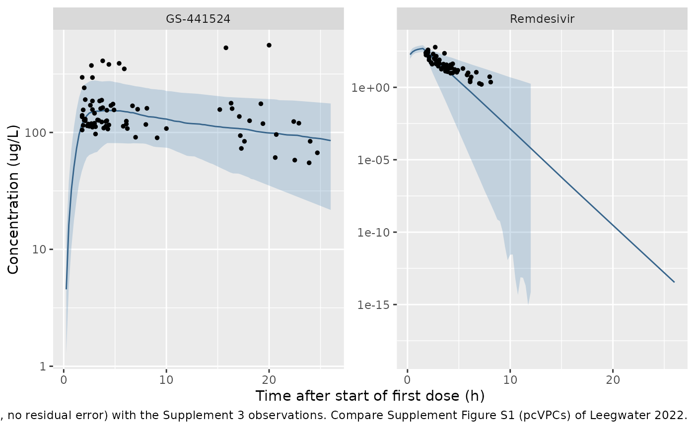
# The observed GS-441524 concentrations should sit mostly inside the
# simulated 90% interval at their sampling times. A mis-specified clearance,
# volume or unit moves the band by tens of percent and fails this; the bound
# is wide because there are only 78 GS-441524 observations from 16 patients.
gs_band <- vpc |> dplyr::filter(analyte == "GS-441524")
gs_obs <- observed |>
  dplyr::filter(analyte == "GS-441524") |>
  dplyr::mutate(
    lo = approx(gs_band$time, gs_band$lo, time)$y,
    hi = approx(gs_band$time, gs_band$hi, time)$y,
    inside = conc_ugL >= lo & conc_ugL <= hi
  )
frac_inside <- mean(gs_obs$inside)
frac_inside
#> [1] 0.8846154
stopifnot(frac_inside > 0.7)
PKNCA: first dose of 200 mg
Non-compartmental analysis of a single 200-mg dose (1.5-h infusion) for each analyte, observed for 168 h so that the GS-441524 terminal phase is captured. The published values are the half-lives (0.48 h and 26.6 h), the GS-441524 Tmax (3.7 h) and the first-24-h average GS-441524 maximum (173 ug/L).
rxode2::rxSetSeed(1)
set.seed(1)
n_nca <- 200L
nca_times <- c(0, seq(0.1, 4, by = 0.1), seq(4.25, 12, by = 0.25), seq(13, 168, by = 1))
ev_nca <- dplyr::bind_rows(lapply(seq_len(n_nca), function(i) {
  make_events(i, 0, 200, 1.5, 94, nca_times)
}))
sim_nca <- as.data.frame(rxode2::rxSolve(mod, ev_nca))

conc_long <- sim_nca |>
  dplyr::select(id, time, Cc, Cc_gs441524) |>
  tidyr::pivot_longer(c(Cc, Cc_gs441524), names_to = "treatment", values_to = "Cc") |>
  dplyr::mutate(treatment = ifelse(treatment == "Cc", "Remdesivir", "GS-441524")) |>
  dplyr::filter(!is.na(Cc))

# Integrator noise: remdesivir decays by ~e^-200 over 168 h, so its tail is
# numerically zero. Assert any undershoot is noise, floor it, and drop the
# numerically-zero tail after the peak so the half-life fit does not follow it.
stopifnot(all(conc_long$Cc >= -1e-6 * max(conc_long$Cc)))
conc_long <- conc_long |>
  dplyr::mutate(Cc = pmax(Cc, 0)) |>
  dplyr::group_by(treatment, id) |>
  dplyr::filter(time <= time[which.max(Cc)] | Cc >= 1e-6 * max(Cc)) |>
  dplyr::ungroup()

conc_long <- dplyr::bind_rows(
  conc_long,
  conc_long |> dplyr::distinct(treatment, id) |> dplyr::mutate(time = 0, Cc = 0)
) |>
  dplyr::distinct(treatment, id, time, .keep_all = TRUE) |>
  dplyr::arrange(treatment, id, time)

dose_df <- ev_nca |>
  dplyr::filter(evid == 1) |>
  dplyr::select(id, time, amt, dur) |>
  tidyr::crossing(treatment = c("Remdesivir", "GS-441524"))

conc_obj <- PKNCA::PKNCAconc(conc_long, Cc ~ time | treatment + id)
dose_obj <- PKNCA::PKNCAdose(dose_df, amt ~ time | treatment + id,
                             route = "intravascular", duration = "dur")
intervals <- data.frame(
  start = 0, end = Inf,
  cmax = TRUE, tmax = TRUE, half.life = TRUE, aucinf.obs = TRUE
)
nca_res <- PKNCA::pk.nca(PKNCA::PKNCAdata(conc_obj, dose_obj, intervals = intervals))
published <- tibble::tribble(
  ~treatment,   ~cmax, ~tmax, ~half.life,
  "Remdesivir", NA,    NA,    0.48,
  "GS-441524",  0.173, 3.7,   26.6
)
cmp <- nlmixr2lib::ncaComparisonTable(
  simulated = nca_res,
  reference = published,
  by = "treatment",
  units = c(cmax = "mg/L", tmax = "h", half.life = "h"),
  tolerance_pct = 20
)
knitr::kable(cmp, caption = "Simulated (median) vs. published NCA. * differs from reference by >20%.")| NCA parameter | treatment | Reference | Simulated | % diff |
|---|---|---|---|---|
| Cmax (mg/L) | Remdesivir | — | 0.482 | — |
| Cmax (mg/L) | GS-441524 | 0.173 | 0.156 | -9.9% |
| Tmax (h) | Remdesivir | — | 1.5 | — |
| Tmax (h) | GS-441524 | 3.7 | 3.95 | +6.8% |
| t½ (h) | Remdesivir | 0.48 | 0.547 | +14.0% |
| t½ (h) | GS-441524 | 26.6 | 27.7 | +4.2% |
The paper’s 173 ug/L is described as the average first-day GS-441524 maximum; the table above pools by median. The mean of the simulated individual maxima is checked directly below. With 42.9% IIV on the GS-441524 volume, the mean of the maxima exceeds their median by about exp(0.184 / 2) - 1 = 10%, which is the gap between the two.
nca_df <- as.data.frame(nca_res)
pp <- function(trt, param) {
  v <- nca_df$PPORRES[nca_df$treatment == trt & nca_df$PPTESTCD == param]
  stopifnot(length(v) == n_nca)
  v
}
gs_cmax_24 <- sim_nca |>
  dplyr::filter(time <= 24) |>
  dplyr::group_by(id) |>
  dplyr::summarise(cmax = max(Cc_gs441524), .groups = "drop")
c(
  mean_gs_cmax_ugL = 1000 * mean(gs_cmax_24$cmax),
  median_rdv_t12 = median(pp("Remdesivir", "half.life")),
  median_gs_t12 = median(pp("GS-441524", "half.life"))
)
#> mean_gs_cmax_ugL   median_rdv_t12    median_gs_t12
#>       170.689855         0.547079        27.714117
# Instrument check: PKNCA's terminal half-life against each subject's own
# log(2) / k from the same drawn parameters. Same draw on both sides, so the
# difference is numerical only and a tight bound is correct.
true_t12 <- sim_nca |>
  dplyr::group_by(id) |>
  dplyr::summarise(
    rdv = log(2) / (kel[1] + kform[1]),
    gs = log(2) / kel_gs441524[1],
    .groups = "drop"
  )
stopifnot(
  max(abs(pp("Remdesivir", "half.life") / true_t12$rdv - 1)) < 0.01,
  max(abs(pp("GS-441524", "half.life") / true_t12$gs - 1)) < 0.01
)

# Centre-of-distribution checks against the paper. MC standard error of the
# mean Cmax with n = 200 and ~45% CV is about 3%, so 12% leaves >3 SE while a
# mis-transcribed volume or dose still fails it. The median individual
# half-life has a combined eta SD of ~0.62 on the log scale for both
# analytes, so its n = 200 standard error is ~6%; one 16-thread draw landed
# 14% above 0.48 h (2.5 SE), so the bound is 25% (> 3 SE). The typical-value
# half-lives are already pinned tightly in the structural-check chunk.
stopifnot(
  abs(1000 * mean(gs_cmax_24$cmax) / 173 - 1) < 0.12,
  abs(median(pp("Remdesivir", "half.life")) / 0.48 - 1) < 0.25,
  abs(median(pp("GS-441524", "half.life")) / 26.6 - 1) < 0.25
)
A gap of 10-15% in a half-life row of the table reflects which 200
subjects were drawn, not the model: the PKNCA estimate matches each
subject’s own log(2) / k, and the typical-value half-lives
(0.478 h and 26.6 h) match the paper.
Monte Carlo dosing simulations (Figures 1-3)
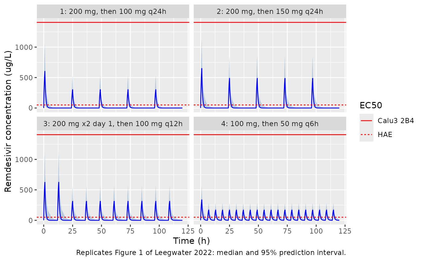
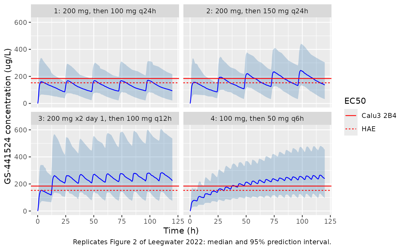
The paper simulated four 5-day regimens in a typical patient with eGFR 94 mL/min/1.73 m^2 (Methods, ‘Probability of target attainment’):
- 200 mg on day 1, then 100 mg once daily (licensed regimen);
- 200 mg on day 1, then 150 mg once daily for 4 days;
- 200 mg twice on day 1, then 100 mg every 12 h, 5 days in total;
- 100 mg loading dose, then 50 mg every 6 h, 5 days in total.
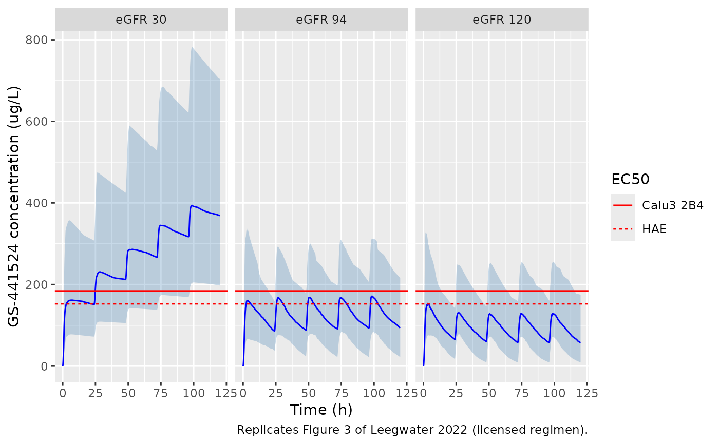
and the licensed regimen at eGFR 30, 94 and 120 mL/min/1.73 m^2. The target was reaching the protein-binding-corrected in vitro EC50 at any time during therapy: 1,406 ug/L (Calu3 2B4 cells) and 50.2 ug/L (human airway epithelial cells) for remdesivir; 184.3 ug/L and 152.6 ug/L, respectively, for GS-441524. The paper used 1,000 virtual patients per scenario; this vignette uses 200 per scenario and a 1-h infusion.
regimens <- list(
  "1: 200 mg, then 100 mg q24h" = list(t = c(0, 24, 48, 72, 96), a = c(200, rep(100, 4))),
  "2: 200 mg, then 150 mg q24h" = list(t = c(0, 24, 48, 72, 96), a = c(200, rep(150, 4))),
  "3: 200 mg x2 day 1, then 100 mg q12h" = list(t = c(0, 12, seq(24, 108, by = 12)), a = c(200, 200, rep(100, 8))),
  "4: 100 mg, then 50 mg q6h" = list(t = seq(0, 114, by = 6), a = c(100, rep(50, 19)))
)
scenarios <- dplyr::bind_rows(
  tibble(scenario = names(regimens), regimen = names(regimens), crcl = 94),
  tibble(scenario = paste0("eGFR ", c(30, 120)), regimen = names(regimens)[1], crcl = c(30, 120))
)
n_mc <- 200L
mc_times <- seq(0, 120, by = 0.1)
ev_mc <- dplyr::bind_rows(lapply(seq_len(nrow(scenarios)), function(k) {
  r <- regimens[[scenarios$regimen[k]]]
  dplyr::bind_rows(lapply(seq_len(n_mc), function(i) {
    make_events((k - 1L) * n_mc + i, r$t, r$a, 1, scenarios$crcl[k], mc_times)
  })) |>
    dplyr::mutate(scenario = scenarios$scenario[k])
}))
stopifnot(!anyDuplicated(unique(ev_mc[, c("id", "time", "evid")])))

rxode2::rxSetSeed(2022)
sim_mc <- as.data.frame(rxode2::rxSolve(mod, ev_mc, keep = "scenario"))
ec50 <- tibble::tribble(
  ~analyte,     ~ec50_ugL, ~cell,
  "Remdesivir", 1406,      "Calu3 2B4",
  "Remdesivir", 50.2,      "HAE",
  "GS-441524",  184.3,     "Calu3 2B4",
  "GS-441524",  152.6,     "HAE"
)
band <- sim_mc |>
  dplyr::filter(scenario %in% names(regimens)) |>
  dplyr::select(scenario, id, time, Cc, Cc_gs441524) |>
  tidyr::pivot_longer(c(Cc, Cc_gs441524), names_to = "analyte", values_to = "conc") |>
  dplyr::mutate(analyte = ifelse(analyte == "Cc", "Remdesivir", "GS-441524")) |>
  dplyr::group_by(scenario, analyte, time) |>
  dplyr::summarise(
    lo = 1000 * quantile(conc, 0.025),
    med = 1000 * median(conc),
    hi = 1000 * quantile(conc, 0.975),
    .groups = "drop"
  )

for (a in c("Remdesivir", "GS-441524")) {
  p <- ggplot(dplyr::filter(band, analyte == a), aes(time, med)) +
    geom_ribbon(aes(ymin = lo, ymax = hi), fill = "steelblue", alpha = 0.3) +
    geom_line(colour = "blue") +
    geom_hline(
      data = dplyr::filter(ec50, analyte == a),
      aes(yintercept = ec50_ugL, linetype = cell), colour = "red"
    ) +
    facet_wrap(~scenario) +
    labs(
      x = "Time (h)", y = paste(a, "concentration (ug/L)"), linetype = "EC50",
      caption = sprintf(
        "Replicates Figure %d of Leegwater 2022: median and 95%% prediction interval.",
        ifelse(a == "Remdesivir", 1, 2)
      )
    )
  print(p)
}
sim_mc |>
  dplyr::filter(scenario %in% c("eGFR 30", names(regimens)[1], "eGFR 120")) |>
  dplyr::mutate(
    egfr = factor(
      ifelse(scenario == names(regimens)[1], "eGFR 94", scenario),
      levels = c("eGFR 30", "eGFR 94", "eGFR 120")
    )
  ) |>
  dplyr::group_by(egfr, time) |>
  dplyr::summarise(
    lo = 1000 * quantile(Cc_gs441524, 0.025),
    med = 1000 * median(Cc_gs441524),
    hi = 1000 * quantile(Cc_gs441524, 0.975),
    .groups = "drop"
  ) |>
  ggplot(aes(time, med)) +
  geom_ribbon(aes(ymin = lo, ymax = hi), fill = "steelblue", alpha = 0.3) +
  geom_line(colour = "blue") +
  geom_hline(
    data = dplyr::filter(ec50, analyte == "GS-441524"),
    aes(yintercept = ec50_ugL, linetype = cell), colour = "red"
  ) +
  facet_wrap(~egfr) +
  labs(
    x = "Time (h)", y = "GS-441524 concentration (ug/L)", linetype = "EC50",
    caption = "Replicates Figure 3 of Leegwater 2022 (licensed regimen)."
  )
Probability of target attainment
pta_sim <- sim_mc |>
  dplyr::group_by(scenario, id) |>
  dplyr::summarise(
    rdv_max = 1000 * max(Cc), gs_max = 1000 * max(Cc_gs441524),
    .groups = "drop"
  ) |>
  dplyr::group_by(scenario) |>
  dplyr::summarise(
    `Remdesivir 1406` = 100 * mean(rdv_max >= 1406),
    `Remdesivir 50.2` = 100 * mean(rdv_max >= 50.2),
    `GS-441524 184.3` = 100 * mean(gs_max >= 184.3),
    `GS-441524 152.6` = 100 * mean(gs_max >= 152.6),
    .groups = "drop"
  ) |>
  tidyr::pivot_longer(-scenario, names_to = "target", values_to = "simulated")

# Results, 'Monte Carlo simulations'. The paper prints GS-441524 PTAs at
# both EC50s for regimens 1-4, but only the 184.3 ug/L PTA for the eGFR
# scenarios.
r <- names(regimens)
pta_paper <- tibble::tribble(
  ~scenario,   ~target,           ~paper,
  r[1],        "Remdesivir 1406", 0.7,
  r[1],        "Remdesivir 50.2", 100,
  r[2],        "Remdesivir 1406", 0.7,
  r[2],        "Remdesivir 50.2", 100,
  r[3],        "Remdesivir 1406", 0.7,
  r[3],        "Remdesivir 50.2", 100,
  r[4],        "Remdesivir 1406", 0.0,
  r[4],        "Remdesivir 50.2", 100,
  r[1],        "GS-441524 152.6", 74.8,
  r[1],        "GS-441524 184.3", 51.9,
  r[2],        "GS-441524 152.6", 93.8,
  r[2],        "GS-441524 184.3", 81.6,
  r[3],        "GS-441524 152.6", 99.3,
  r[3],        "GS-441524 184.3", 94.7,
  r[4],        "GS-441524 152.6", 89.0,
  r[4],        "GS-441524 184.3", 78.7,
  "eGFR 30",   "GS-441524 184.3", 99.4,
  "eGFR 120",  "GS-441524 184.3", 35.9
)
pta_cmp <- pta_paper |>
  dplyr::left_join(pta_sim, by = c("scenario", "target")) |>
  dplyr::mutate(difference = simulated - paper)
stopifnot(nrow(pta_cmp) == 18L, !anyNA(pta_cmp$simulated))

pta_cmp |>
  dplyr::rename(
    "Scenario" = scenario, "Target (ug/L)" = target,
    "Paper PTA (%)" = paper, "Simulated PTA (%)" = simulated,
    "Difference (points)" = difference
  ) |>
knitr::kable(digits = 1, caption = "Probability of reaching the EC50 at any time during 5 days of therapy.")| Scenario | Target (ug/L) | Paper PTA (%) | Simulated PTA (%) | Difference (points) |
|---|---|---|---|---|
| 1: 200 mg, then 100 mg q24h | Remdesivir 1406 | 0.7 | 0.5 | -0.2 |
| 1: 200 mg, then 100 mg q24h | Remdesivir 50.2 | 100.0 | 100.0 | 0.0 |
| 2: 200 mg, then 150 mg q24h | Remdesivir 1406 | 0.7 | 0.5 | -0.2 |
| 2: 200 mg, then 150 mg q24h | Remdesivir 50.2 | 100.0 | 100.0 | 0.0 |
| 3: 200 mg x2 day 1, then 100 mg q12h | Remdesivir 1406 | 0.7 | 0.0 | -0.7 |
| 3: 200 mg x2 day 1, then 100 mg q12h | Remdesivir 50.2 | 100.0 | 100.0 | 0.0 |
| 4: 100 mg, then 50 mg q6h | Remdesivir 1406 | 0.0 | 0.0 | 0.0 |
| 4: 100 mg, then 50 mg q6h | Remdesivir 50.2 | 100.0 | 100.0 | 0.0 |
| 1: 200 mg, then 100 mg q24h | GS-441524 152.6 | 74.8 | 75.0 | 0.2 |
| 1: 200 mg, then 100 mg q24h | GS-441524 184.3 | 51.9 | 54.0 | 2.1 |
| 2: 200 mg, then 150 mg q24h | GS-441524 152.6 | 93.8 | 92.5 | -1.3 |
| 2: 200 mg, then 150 mg q24h | GS-441524 184.3 | 81.6 | 82.5 | 0.9 |
| 3: 200 mg x2 day 1, then 100 mg q12h | GS-441524 152.6 | 99.3 | 99.5 | 0.2 |
| 3: 200 mg x2 day 1, then 100 mg q12h | GS-441524 184.3 | 94.7 | 95.0 | 0.3 |
| 4: 100 mg, then 50 mg q6h | GS-441524 152.6 | 89.0 | 90.5 | 1.5 |
| 4: 100 mg, then 50 mg q6h | GS-441524 184.3 | 78.7 | 81.0 | 2.3 |
| eGFR 30 | GS-441524 184.3 | 99.4 | 98.5 | -0.9 |
| eGFR 120 | GS-441524 184.3 | 35.9 | 39.0 | 3.1 |
# Binomial SE of a PTA near 50% is 3.5 points at n = 200 and 1.6 points
# for the paper's n = 1,000; with 1,000-2,000 subjects per scenario the
# model reproduces every published cell within about 4 points (largest gap
# regimen 4, where the paper's numbers sit ~3-4 points below). 15 points
# per cell is > 3 combined SE beyond that, and 7 points on the mean
# absolute difference catches a shifted clearance, volume or eGFR exponent,
# which moves these PTAs by tens of points.
stopifnot(
  max(abs(pta_cmp$difference)) < 15,
  mean(abs(pta_cmp$difference)) < 7
)
Assumptions and deviations
-
Renal arm added to, not carved out of, the metabolic
clearance. The Results describe nonmetabolic remdesivir
clearance as fixed to “10% of the total remdesivir clearance”, but the
control stream codes
CL = 0.1 * CLtoM, i.e. 10% of the metabolic clearance, so total clearance is 1.1 x 207 = 227.7 L/h and the renal arm is 9.1% of the total. The code is what was fitted, and it is the reading that reproduces the reported 0.48 h half-life (the alternative, 207 L/h total, gives 0.53 h). The model therefore estimateslcl_metand fixes the ratioclrat_gs441524 = 10; the single remdesivir eta scales both arms, as in the control stream. -
Parameter labels in the control stream. The control
stream’s comments call
THETA(1)andOMEGA(1)the “non metabolism” clearance, but the code uses them for the metabolic (GS-441524-forming) arm and Table 2 labels them ‘Metabolic CL’ and ‘Remdesivir nonrenal CL’. The model follows the code and Table 2. -
No molecular-weight conversion. The source
transfers remdesivir mass directly into the GS-441524 compartment
(ADVAN5
K12) and fits GS-441524 in mg/L, so the GS-441524 volume and clearance are apparent values that absorb the molar-mass ratio (602.6 / 291.3 g/mol) and any fraction not converted. GS-441524 concentrations are predicted correctly in mass units; the GS-441524 amount state is not a true amount. A dose must be given in mg of remdesivir. -
Residual error is additive on the linear scale, per
the control stream (
Y = IPRED + W*EPS(1),$SIGMA 1 FIX), although the Methods state that residual variability was assumed log-normal. The Results also say “an additive-error model was used”, consistent with the code. - Infusion duration. Patients were infused over 1 to 2 h; the paper does not state the duration used in the Monte Carlo simulations. The dosing simulations here use 1 h; the GS-441524 PTAs change by less than one point between 1 and 2 h, and the remdesivir 1,406 ug/L PTA, already below 1%, falls to zero with longer infusions.
-
PTA definition. The target is read as the
individual maximum (no residual error) over 5 days reaching the
protein-binding-corrected EC50, per the Methods (“reaching the EC50 at
any point during therapy was sufficient”). The paper’s EC50s are already
corrected to total plasma concentrations, so they are compared to
CcandCc_gs441524directly. - Virtual cohort. The paper’s simulations used a typical patient’s covariates (eGFR fixed) with between-subject variability; this vignette does the same, with 200 rather than 1,000 subjects per scenario. The first-day VPC samples eGFR log-normally around the median (94) within the observed range (8-119), as a stand-in for the unpublished individual covariates.
-
Covariates tested but not retained (age, weight
with and without allometric scaling, BSA, BMI, CRP, ALT) are listed in
the model’s
covariatesDataExcludedmetadata. - Observed data. Supplement 3 lists 78 sampling times from 16 patients (patient 14 has no rows) where the Results report 84 samples from 17 patients; the 78 listed rows are used as published.
- Below-quantification data. The paper modelled remdesivir below-LOQ data with the all-data method; this has no bearing on simulation. Supplement 3 values marked ‘BLD’ are omitted from the VPC overlay.
- No erratum or correction notice was found for this article (Europe PMC, checked 2026-10-01).