Benznidazole in T. cruzi-infected mice (Assmus 2025)
Source:vignettes/articles/Assmus_2025_benznidazole_mouse.Rmd
Assmus_2025_benznidazole_mouse.RmdModel and source
- Citation: Assmus F, Adehin A, Hoglund RM, Fortes Francisco A, Lewis MD, Kelly JM, Charman SA, White KL, Shackleford DM, Escudie F, Chatelain E, Scandale I, Tarning J. Pharmacokinetic-pharmacodynamic modeling of benznidazole and its antitrypanosomal activity in a murine model of chronic Chagas disease. PLoS Negl Trop Dis. 2025;19(5):e0012968. doi:10.1371/journal.pntd.0012968.
- Description: Preclinical (mouse). One-compartment population PK model with first-order absorption for benznidazole in female BALB/c mice, with a priori allometric scaling on CL/F (exponent 0.75) and Vc/F (exponent 1.0) centred on 19.4 g, and a power-function effect of the administered mg/kg dose on the absorption rate constant (KA falls from 5.11 to 0.86 1/h between 10 and 100 mg/kg). The model carries two PK/PD index accumulator states – cumulative plasma AUC and cumulative time above the protein-binding-corrected in vitro IC90 against Trypanosoma cruzi amastigotes (6.427 ug/mL) – which drive the paper’s binary univariate logistic exposure-response models for sterile parasitological cure in chronically infected mice, measured by in vivo and ex vivo bioluminescence imaging.
- Article: https://doi.org/10.1371/journal.pntd.0012968
- Supporting information (S1 Code holds the NONMEM control stream of the final PK model): https://journals.plos.org/plosntds/article?id=10.1371/journal.pntd.0012968#sec023
This is a preclinical, two-layer model. A population PK layer was estimated in uninfected satellite mice; the resulting typical profiles were then used to generate exposure metrics that drive a binary logistic exposure-response layer for sterile parasitological cure in a separate cohort of chronically infected mice.
Population
The PK layer was estimated from 52 uninfected female BALB/c mice given a single oral gavage dose of benznidazole at 10 mg/kg (n = 16), 30 mg/kg (n = 18) or 100 mg/kg (n = 18). Mice weighed 18.1-21.6 g at dosing (median 19.4 g, SD 0.92 g). Sampling was sparse: 1-3 samples per mouse at nominal times of 0.25, 0.5, 1, 2, 4, 4.5, 6, 8, 10, 12, 14, 16 and 24 h. Of 110 collected samples, two outliers were excluded and data were censored beyond 8 h (10 mg/kg) and 12 h (30 mg/kg) because all later concentrations were below the 5 ng/mL LLOQ; 90 quantifiable samples entered the final fit. Estimation used NONMEM 7.4 with FOCE-I on natural-log-transformed concentrations, and parameter precision came from sampling importance resampling.
The exposure-response layer was fitted in a separate cohort of 118 female BALB/c mice with chronic-stage Trypanosoma cruzi CL Brener infection (1000 bioluminescent blood trypomastigotes; chronic stage reached 50-70 days post-infection). These mice weighed 20.5-28.1 g (median 25 g) and received 10, 20, 30, 50 or 100 mg/kg per administration for 5, 10 or 20 days across ten regimens (Table 1 of the source). Parasitological cure – absence of bioluminescence on both in vivo and ex vivo imaging after cyclophosphamide immunosuppression – was achieved in 83 of 118 mice.
The same information is available programmatically via the model’s
population metadata
(readModelDb("Assmus_2025_benznidazole_mouse")()$population).
Source trace
The per-parameter origin is recorded as an in-file comment next to
each ini() entry in
inst/modeldb/specificDrugs/Assmus_2025_benznidazole_mouse.R.
The table below collects them in one place for review. “S1 Code” is the
NONMEM control stream of the final PK model, published as supporting
information.
| Equation / parameter | Value | Source location |
|---|---|---|
lka |
log(2.18) 1/h |
Table 2: K_A = 2.18 (RSE 15.9%, 95% CI 1.65-3.03); S1 Code
$THETA 3
|
lcl |
log(0.0106) L/h |
Table 2: CL/F = 10.6 mL/h (RSE 5.6%, 95% CI 9.62-11.88); S1 Code
$THETA 1
|
lvc |
log(0.0197) L |
Table 2: V_C/F = 19.7 mL (RSE 8.2%, 95% CI 17.05-23.18); S1 Code
$THETA 2
|
lfdepot |
fixed(log(1)) |
Methods: “Relative bioavailability (F, fixed to unity for the
population)”; S1 Code $THETA 4 = “1 FIX” |
e_wt_cl |
fixed(0.75) |
Methods: allometric function on clearance, exponent 0.75, a priori;
S1 Code TVCL = THETA(1)*((WT/0.0194)**0.75)
|
e_wt_vc |
fixed(1.0) |
Methods: allometric function on volume, exponent 1, a priori; S1
Code TVV2 = THETA(2)*((WT/0.0194)**1.00)
|
e_dose_ka |
-0.775 |
Table 2: theta_Dose = -0.775 (RSE 13.3%, 95% CI -0.977 to -0.583);
S1 Code $THETA 5
|
etalcl |
~ 0.0298 |
S1 Code $OMEGA IIV_CL = 0.0298; Table 2 reports the
back-transform 17.4 %CV |
etalvc |
~ 0.0271 |
S1 Code $OMEGA IIV_V2 = 0.0271; Table 2 reports the
back-transform 16.6 %CV |
expSd |
sqrt(0.122) |
Table 2: sigma = 0.122 (95% CI 0.087-0.188); S1 Code
$SIGMA 0.122 (a variance) |
mic |
fixed(6.427) ug/mL |
Table 1 footnote: “T>IC90, Time above IC90 in plasma (6.427 ug/mL…)”; Methods: IC90,plasma = 24.7 uM; derivation in S1 Text |
logite0_cure_auc |
-2.170 |
Table 4, AUCinf column: Intercept (SE 0.566) |
e_auc_cure |
0.0033 |
Table 4, AUCinf column: LogOdds (SE 0.0006) |
logite0_cure_tmic |
-1.859 |
Table 4, T>IC90 column: Intercept (SE 0.521) |
e_tmic_cure |
1.497 |
Table 4, T>IC90 column: LogOdds (SE 0.289) |
| Reference weight 0.0194 kg | n/a | Methods: allometry “centered on the median weight of mice in the
satellite PK study (19.4 g)”; S1 Code (WT/0.0194)
|
| Reference dose 30 mg/kg | n/a | Methods: “individual doses centered on the median dose (30 mg/kg)”;
S1 Code (DOSE_PER_KG/30)
|
d/dt(depot), d/dt(central)
|
n/a | Results: one-compartment disposition with first-order absorption; S1
Code ADVAN5 TRANS1, COMP(1) ->
COMP(2), K12 = KA,
K20 = CL/V2
|
ka <- exp(lka) * (DOSE_BZN_MGKG/30)^e_dose_ka |
n/a | Methods (power function on dose, centered on the median); S1 Code
COV1 = (DOSE_PER_KG/30)**THETA(5),
TVKA = THETA(3)*COV1
|
Cc ~ lnorm(expSd) |
n/a | Methods: “additive error on the log-transformed observed
concentrations”; S1 Code
$ERROR Y = LOG(IPRED) + EPS(1)
|
d/dt(auc_total) <- Cc |
n/a | Methods, “Simulation of benznidazole exposure”: cumulative AUC to infinity extracted from simulated profiles |
d/dt(t_above_mic) <- (Cc >= mic)/24 |
n/a | Methods: “the time above the target concentration in mice (T>IC90) … was calculated”; reported in days (Table 1) |
pcure_* <- 1/(1 + exp(-(logite0_* + e_*))) |
n/a | Equation 1: logit(p) = beta0 + beta1*x
|
mod <- readModelDb("Assmus_2025_benznidazole_mouse")Part 1 – Population PK in satellite mice
Virtual cohort
Original observed data are not publicly available. The satellite cohort below reproduces the published design: three single-dose groups, weights drawn to match the reported 18.1-21.6 g range with a 19.4 g median and 0.92 g SD. The physical dose is computed per mouse from its own weight, exactly as the study did (“Doses, individually adjusted according to each mouse’s weight”).
set.seed(20250513)

n_per_arm <- 200L  # cap is 200 participants per arm

make_pk_arm <- function(mgkg, n, id_offset) {
  wt <- pmin(pmax(rnorm(n, mean = 0.0194, sd = 0.00092), 0.0181), 0.0216)
  subj <- tibble(
    id            = id_offset + seq_len(n),
    WT            = wt,
    DOSE_BZN_MGKG = mgkg,
    arm           = paste0(mgkg, " mg/kg")
  )
  doses <- subj |>
    mutate(time = 0, evid = 1L, amt = DOSE_BZN_MGKG * WT, cmt = "depot")
  obs <- subj |>
    tidyr::crossing(time = seq(0, 24, by = 0.25)) |>
    mutate(evid = 0L, amt = NA_real_, cmt = "central")
  bind_rows(doses, obs) |> arrange(id, time, desc(evid))
}

events_pk <- bind_rows(
  make_pk_arm(10,  n_per_arm, id_offset = 0L),
  make_pk_arm(30,  n_per_arm, id_offset = 1000L),
  make_pk_arm(100, n_per_arm, id_offset = 2000L)
)
# No (id, time, evid) triple may repeat: `unique()` must NOT be applied first,
# or the check is vacuous (deduplicating before asking for duplicates).
stopifnot(!anyDuplicated(events_pk[, c("id", "time", "evid")]))
Simulation
sim_pk <- rxode2::rxSolve(
  mod,
  events = events_pk,
  keep   = c("arm", "WT", "DOSE_BZN_MGKG")
) |>
  as.data.frame()
#> ℹ parameter labels from comments will be replaced by 'label()'

stopifnot(dplyr::n_distinct(sim_pk$id) == 3L * n_per_arm)
stopifnot(all(sim_pk$Cc >= 0))
Replicating Figure 1 (visual predictive check)
# Replicates Figure 1 of Assmus 2025: simulated 5th / 50th / 95th percentiles
# of benznidazole plasma concentration by dose group, with the 5 ng/mL LLOQ.
sim_pk |>
  filter(!is.na(Cc), time > 0) |>
  mutate(arm = factor(arm, levels = c("10 mg/kg", "30 mg/kg", "100 mg/kg"))) |>
  group_by(arm, time) |>
  summarise(
    Q05 = quantile(sim, 0.05),
    Q50 = quantile(sim, 0.50),
    Q95 = quantile(sim, 0.95),
    .groups = "drop"
  ) |>
  ggplot(aes(time, Q50)) +
  geom_ribbon(aes(ymin = Q05, ymax = Q95), alpha = 0.25, fill = "steelblue") +
  geom_line(colour = "red") +
  geom_hline(yintercept = 0.005, linetype = "dashed") +
  facet_wrap(~arm) +
  scale_y_log10() +
  labs(
    x = "Time after dose (h)", y = "Benznidazole (ug/mL)",
    title = "Figure 1 - simulated concentration-time profiles by dose group",
    caption = paste(
      "Replicates Figure 1 of Assmus 2025. Red = median, band = 5th-95th",
      "percentile of the simulated observations (residual error included).",
      "Dashed line = LLOQ (0.005 ug/mL)."
    )
  )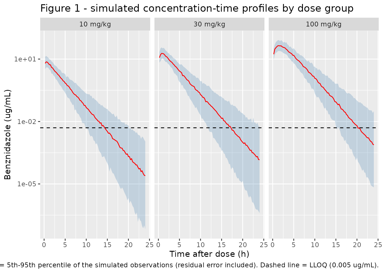
The dose-dependent absorption is visible directly: the peak shifts
later and broadens as the dose rises, because ka falls from
5.11 to 0.86 1/h between 10 and 100 mg/kg.
tibble(`Dose (mg/kg)` = c(10, 30, 100)) |>
  mutate(
    `KA, model (1/h)`     = round(2.18 * (`Dose (mg/kg)` / 30)^(-0.775), 2),
    `KA, published (1/h)` = c(5.11, 2.18, 0.86)
  ) |>
  knitr::kable(caption = paste(
    "Absorption rate constant by dose level. Published values from the",
    "Results section, 'Pharmacokinetics of benznidazole'."
))| Dose (mg/kg) | KA, model (1/h) | KA, published (1/h) |
|---|---|---|
| 10 | 5.11 | 5.11 |
| 30 | 2.18 | 2.18 |
| 100 | 0.86 | 0.86 |
PKNCA validation
sim_nca <- sim_pk |>
  filter(!is.na(Cc)) |>
  select(id, time, Cc, arm)

# Guarantee a time = 0 row per (id, arm); pre-dose Cc = 0 for oral dosing.
sim_nca <- bind_rows(
  sim_nca,
  sim_nca |> distinct(id, arm) |> mutate(time = 0, Cc = 0)
) |>
  distinct(id, arm, time, .keep_all = TRUE) |>
  arrange(id, arm, time)

stopifnot(nrow(sim_nca) > 0, all(sim_nca$Cc >= 0))

conc_obj <- PKNCA::PKNCAconc(sim_nca, Cc ~ time | arm + id)

dose_df <- events_pk |>
  filter(evid == 1L) |>
  select(id, time, amt, arm)

dose_obj <- PKNCA::PKNCAdose(dose_df, amt ~ time | arm + id)

intervals <- data.frame(
  start      = 0,
  end        = Inf,
  cmax       = TRUE,
  tmax       = TRUE,
  aucinf.obs = TRUE,
  half.life  = TRUE
)

nca_res <- PKNCA::pk.nca(PKNCA::PKNCAdata(conc_obj, dose_obj, intervals = intervals))
Comparison against the published secondary PK parameters
S2 Table of the source reports model-derived secondary parameters as median (5th-95th percentile) per dose group.
published <- tibble::tribble(
  ~arm,        ~cmax, ~tmax, ~aucinf.obs, ~half.life,
  "10 mg/kg",    8.0,  0.49,        18.1,       1.23,
  "30 mg/kg",   19.0,  0.86,        57.3,       1.33,
  "100 mg/kg",  44.7,  1.47,       186.0,       1.39
)

cmp <- nlmixr2lib::ncaComparisonTable(
  simulated     = nca_res,
  reference     = published,
  by            = "arm",
  units         = c(cmax = "ug/mL", aucinf.obs = "ug*h/mL",
                    tmax = "h", half.life = "h"),
  tolerance_pct = 20
)

knitr::kable(
  cmp,
  caption = paste(
    "Simulated vs. published secondary PK parameters (S2 Table of Assmus 2025;",
    "medians). * differs from reference by >20%."
  ),
  align = c("l", "l", "r", "r", "r")
)| NCA parameter | arm | Reference | Simulated | % diff |
|---|---|---|---|---|
| Cmax (ug/mL) | 10 mg/kg | 8 | 7.47 | -6.7% |
| Cmax (ug/mL) | 30 mg/kg | 19 | 18.3 | -3.8% |
| Cmax (ug/mL) | 100 mg/kg | 44.7 | 44.4 | -0.7% |
| Tmax (h) | 10 mg/kg | 0.49 | 0.5 | +2.0% |
| Tmax (h) | 30 mg/kg | 0.86 | 0.75 | -12.8% |
| Tmax (h) | 100 mg/kg | 1.47 | 1.5 | +2.0% |
| AUC0-∞ (obs) (ug*h/mL) | 10 mg/kg | 18.1 | 18 | -0.6% |
| AUC0-∞ (obs) (ug*h/mL) | 30 mg/kg | 57.3 | 55.3 | -3.6% |
| AUC0-∞ (obs) (ug*h/mL) | 100 mg/kg | 186 | 184 | -1.0% |
| t½ (h) | 10 mg/kg | 1.23 | 1.28 | +4.3% |
| t½ (h) | 30 mg/kg | 1.33 | 1.34 | +0.5% |
| t½ (h) | 100 mg/kg | 1.39 | 1.33 | -4.6% |
Every parameter agrees with S2 Table well inside the 20% tolerance. The residual few-percent gaps on Cmax and AUCinf reflect the fact that the paper’s medians come from the 52 real mice at their individually measured weights and their actual administered doses (“The exact dose administered to each mouse was calculated based on the measured concentration of the formulation and the animal’s body weight”), whereas this cohort uses nominal mg/kg dose levels.
Part 2 – Simulated exposure in the efficacy regimens
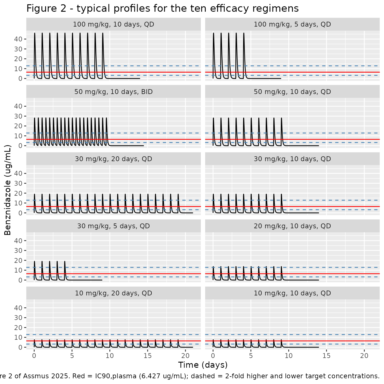
Table 1 of the source reports median exposure metrics for the ten efficacy regimens, simulated from this PK model at the 25 g median weight of the efficacy cohort. Because those are typical-value simulations, the random effects are zeroed here.
mod_typical <- rxode2::zeroRe(mod)
#> ℹ parameter labels from comments will be replaced by 'label()'

wt_eff <- 0.025  # 25 g, median weight of mice in the efficacy studies

regimens <- tibble::tribble(
  ~regimen, ~label,                     ~mgkg, ~n_dose, ~ii,
  "a",      "100 mg/kg, 10 days, QD",     100,      10,  24,
  "b",      "100 mg/kg, 5 days, QD",      100,       5,  24,
  "c",      "50 mg/kg, 10 days, BID",      50,      20,  12,
  "d",      "50 mg/kg, 10 days, QD",       50,      10,  24,
  "e",      "30 mg/kg, 20 days, QD",       30,      20,  24,
  "f",      "30 mg/kg, 10 days, QD",       30,      10,  24,
  "g",      "30 mg/kg, 5 days, QD",        30,       5,  24,
  "h",      "20 mg/kg, 10 days, QD",       20,      10,  24,
  "i",      "10 mg/kg, 20 days, QD",       10,      20,  24,
  "j",      "10 mg/kg, 10 days, QD",       10,      10,  24
)

simulate_regimen <- function(mgkg, n_dose, ii) {
  last_dose <- (n_dose - 1) * ii
  ev <- rxode2::et(amt = mgkg * wt_eff, ii = ii, until = last_dose, cmt = "depot") |>
    rxode2::et(seq(0, last_dose + 120, by = 0.02), cmt = "central")
  d <- as.data.frame(ev)
  d$WT <- wt_eff
  d$DOSE_BZN_MGKG <- mgkg
  rxode2::rxSolve(mod_typical, d, omega = NA, returnType = "data.frame",
                  atol = 1e-10, rtol = 1e-10)
}

sims <- lapply(seq_len(nrow(regimens)), function(i) {
  s <- simulate_regimen(regimens$mgkg[i], regimens$n_dose[i], regimens$ii[i])
  s$regimen <- regimens$regimen[i]
  s$label   <- regimens$label[i]
  s
})
sim_reg <- bind_rows(sims) |> filter(!is.na(Cc))
stopifnot(dplyr::n_distinct(sim_reg$regimen) == nrow(regimens))
Replicating Figure 2 (typical profiles by regimen)
# Replicates Figure 2 of Assmus 2025: median simulated benznidazole profiles
# for each efficacy regimen in a 25 g mouse, against the plasma IC90 and its
# 2-fold bracket.
ic90 <- 6.427

sim_reg |>
  filter(time <= 24 * 21) |>
  mutate(label = factor(label, levels = regimens$label)) |>
  ggplot(aes(time / 24, Cc)) +
  geom_line() +
  geom_hline(yintercept = ic90, colour = "red") +
  geom_hline(yintercept = c(ic90 / 2, ic90 * 2), colour = "steelblue",
             linetype = "dashed") +
  facet_wrap(~label, ncol = 2) +
  labs(
    x = "Time (days)", y = "Benznidazole (ug/mL)",
    title = "Figure 2 - typical profiles for the ten efficacy regimens",
    caption = paste(
      "Replicates Figure 2 of Assmus 2025. Red = IC90,plasma (6.427 ug/mL);",
      "dashed = 2-fold higher and lower target concentrations."
    )
  )
Replicating Table 1 (exposure metrics)
AUC12 and AUC24 are read directly off the
model’s cumulative-AUC state at 12 h and 24 h; AUCinf and
T>IC90 are the terminal values of the
auc_total and t_above_mic states.
at_time <- function(df, tt, col) {
  df[[col]][which.min(abs(df$time - tt))]
}

exposure <- bind_rows(lapply(sims, function(s) {
  tibble(
    regimen = s$regimen[1],
    cmax    = max(s$Cc, na.rm = TRUE),
    auc12   = at_time(s, 12, "auc_total"),
    auc24   = at_time(s, 24, "auc_total"),
    aucinf  = max(s$auc_total),
    tmic    = max(s$t_above_mic),
    p_auc   = max(s$pcure_auc),
    p_tmic  = max(s$pcure_tmic)
  )
}))

published_t1 <- tibble::tribble(
  ~regimen, ~cum_dose, ~r_cmax, ~r_auc12, ~r_auc24, ~r_aucinf, ~r_tmic, ~n_cured, ~n_total,
  "a", 1000, 46.00, 193.4, 194.5, 1945, 2.86, 25, 27,
  "b",  500, 46.08, 195.4, 196.9,  985, 1.44, 17, 17,
  "c", 1000, 28.25,  96.8, 194.1, 1946, 3.95,  6,  6,
  "d",  500, 28.11,  96.9,  97.2,  972, 1.96,  2,  3,
  "e",  600, 19.07,  58.3,  58.6, 1173, 2.85, 23, 29,
  "f",  300, 18.97,  58.1,  58.3,  583, 1.41,  9, 11,
  "g",  150, 19.01,  58.8,  59.1,  295, 0.72,  0,  9,
  "h",  200, 13.70,  38.8,  38.9,  389, 1.01,  0,  4,
  "i",  200,  7.67,  19.5,  19.6,  391, 0.68,  1,  6,
  "j",  100,  7.65,  19.4,  19.4,  194, 0.33,  0,  6
)

tab1 <- exposure |>
  left_join(published_t1, by = "regimen") |>
  left_join(regimens |> select(regimen, label), by = "regimen") |>
  mutate(
    d_cmax   = 100 * (cmax   - r_cmax)   / r_cmax,
    d_auc12  = 100 * (auc12  - r_auc12)  / r_auc12,
    d_auc24  = 100 * (auc24  - r_auc24)  / r_auc24,
    d_aucinf = 100 * (aucinf - r_aucinf) / r_aucinf,
    d_tmic   = 100 * (tmic   - r_tmic)   / r_tmic
  )

tab1 |>
  transmute(
    Regimen                = label,
    `Cmax sim`             = round(cmax, 2),
    `Cmax pub`             = r_cmax,
    `AUC12 sim`            = round(auc12, 1),
    `AUC12 pub`            = r_auc12,
    `AUC24 sim`            = round(auc24, 1),
    `AUC24 pub`            = r_auc24,
    `AUCinf sim`           = round(aucinf, 0),
    `AUCinf pub`           = r_aucinf,
    `T>IC90 sim (d)`       = round(tmic, 2),
    `T>IC90 pub (d)`       = r_tmic
  ) |>
  knitr::kable(caption = paste(
    "Replicates Table 1 of Assmus 2025: simulated median exposures for a 25 g",
    "mouse. Cmax in ug/mL, AUC in ug*h/mL, T>IC90 in days."
))| Regimen | Cmax sim | Cmax pub | AUC12 sim | AUC12 pub | AUC24 sim | AUC24 pub | AUCinf sim | AUCinf pub | T>IC90 sim (d) | T>IC90 pub (d) |
|---|---|---|---|---|---|---|---|---|---|---|
| 100 mg/kg, 10 days, QD | 46.12 | 46.00 | 193.9 | 193.4 | 195.0 | 194.5 | 1950 | 1945 | 2.88 | 2.86 |
| 100 mg/kg, 5 days, QD | 46.12 | 46.08 | 193.9 | 195.4 | 195.0 | 196.9 | 975 | 985 | 1.44 | 1.44 |
| 50 mg/kg, 10 days, BID | 28.23 | 28.25 | 97.2 | 96.8 | 194.7 | 194.1 | 1950 | 1946 | 3.96 | 3.95 |
| 50 mg/kg, 10 days, QD | 28.13 | 28.11 | 97.2 | 96.9 | 97.5 | 97.2 | 975 | 972 | 1.98 | 1.96 |
| 30 mg/kg, 20 days, QD | 19.01 | 19.07 | 58.3 | 58.3 | 58.5 | 58.6 | 1170 | 1173 | 2.85 | 2.85 |
| 30 mg/kg, 10 days, QD | 19.01 | 18.97 | 58.3 | 58.1 | 58.5 | 58.3 | 585 | 583 | 1.43 | 1.41 |
| 30 mg/kg, 5 days, QD | 19.01 | 19.01 | 58.3 | 58.8 | 58.5 | 59.1 | 292 | 295 | 0.71 | 0.72 |
| 20 mg/kg, 10 days, QD | 13.72 | 13.70 | 38.9 | 38.8 | 39.0 | 38.9 | 390 | 389 | 1.02 | 1.01 |
| 10 mg/kg, 20 days, QD | 7.64 | 7.67 | 19.4 | 19.5 | 19.5 | 19.6 | 390 | 391 | 0.67 | 0.68 |
| 10 mg/kg, 10 days, QD | 7.64 | 7.65 | 19.4 | 19.4 | 19.5 | 19.4 | 195 | 194 | 0.33 | 0.33 |
worst <- tab1 |>
  summarise(
    Cmax   = max(abs(d_cmax)),
    AUC12  = max(abs(d_auc12)),
    AUC24  = max(abs(d_auc24)),
    AUCinf = max(abs(d_aucinf)),
    `T>IC90` = max(abs(d_tmic))
  )
knitr::kable(round(worst, 2), caption = "Worst-case absolute % difference vs. Table 1.")| Cmax | AUC12 | AUC24 | AUCinf | T>IC90 |
|---|---|---|---|---|
| 0.4 | 0.81 | 1.02 | 1.02 | 2.2 |
# Every metric must reproduce Table 1 to within 3%. This is a real gate: the
# published values were generated from n = 10 stochastic replicates, so a few
# tenths of a percent of Monte-Carlo noise is expected, but nothing more.
stopifnot(
  nrow(tab1) == 10L,
  max(abs(tab1$d_cmax))   < 3,
  max(abs(tab1$d_auc12))  < 3,
  max(abs(tab1$d_auc24))  < 3,
  max(abs(tab1$d_aucinf)) < 3,
  max(abs(tab1$d_tmic))   < 3
)
All five exposure metrics for all ten regimens reproduce Table 1 to
within 3%. Note the structural signature of the BID regimen (c): its
AUC12 is half that of the matched 100 mg/kg QD regimen (a)
while its AUC24 and AUCinf are the same, and
its T>IC90 is the longest of any regimen (3.95 days) –
splitting the daily dose buys time above target without changing total
exposure.
Part 3 – Exposure-response for parasitological cure
Predicted cure probability by regimen
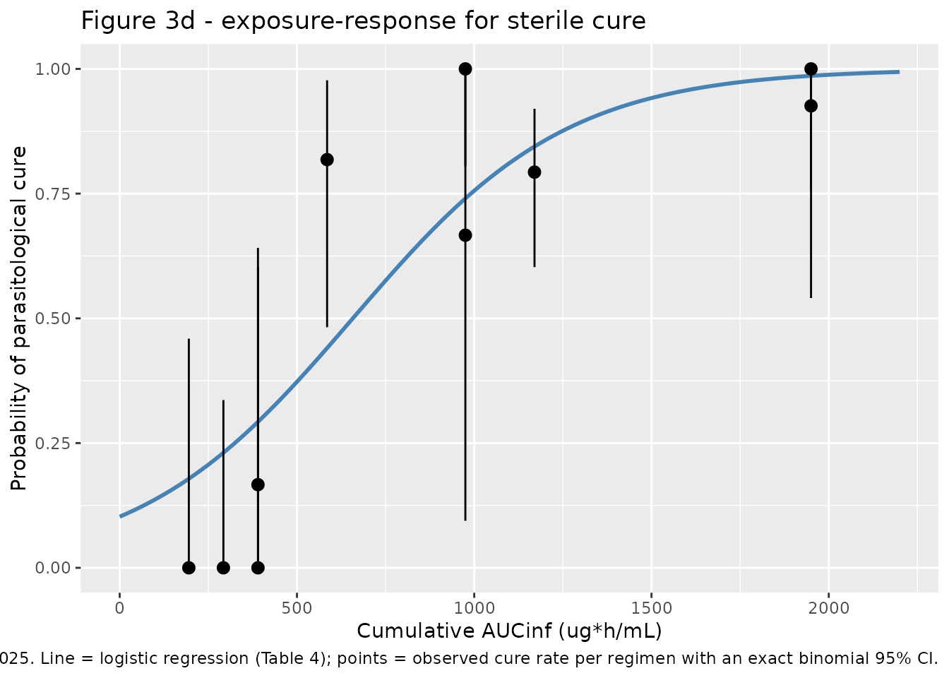
The two logistic models carried inside the model object are evaluated at each regimen’s terminal exposure and compared against the observed cure fraction reported in Table 1.
er <- tab1 |>
  mutate(
    obs_rate = n_cured / n_total,
    lo = mapply(function(x, n) stats::binom.test(x, n)$conf.int[1], n_cured, n_total),
    hi = mapply(function(x, n) stats::binom.test(x, n)$conf.int[2], n_cured, n_total)
  )

er |>
  transmute(
    Regimen                     = label,
    `AUCinf (ug*h/mL)`          = round(aucinf, 0),
    `P(cure) | AUCinf`          = round(p_auc, 3),
    `T>IC90 (days)`             = round(tmic, 2),
    `P(cure) | T>IC90`          = round(p_tmic, 3),
    `Observed cured / total`    = paste0(n_cured, "/", n_total),
    `Observed rate`             = round(obs_rate, 3)
  ) |>
  knitr::kable(caption = paste(
    "Model-predicted probability of sterile parasitological cure vs. the",
    "observed cure rate in each regimen (Table 1 of Assmus 2025)."
))| Regimen | AUCinf (ug*h/mL) | P(cure) | AUCinf | T>IC90 (days) | P(cure) | T>IC90 | Observed cured / total | Observed rate |
|---|---|---|---|---|---|---|
| 100 mg/kg, 10 days, QD | 1950 | 0.986 | 2.88 | 0.921 | 25/27 | 0.926 |
| 100 mg/kg, 5 days, QD | 975 | 0.740 | 1.44 | 0.573 | 17/17 | 1.000 |
| 50 mg/kg, 10 days, BID | 1950 | 0.986 | 3.96 | 0.983 | 6/6 | 1.000 |
| 50 mg/kg, 10 days, QD | 975 | 0.740 | 1.98 | 0.751 | 2/3 | 0.667 |
| 30 mg/kg, 20 days, QD | 1170 | 0.844 | 2.85 | 0.917 | 23/29 | 0.793 |
| 30 mg/kg, 10 days, QD | 585 | 0.440 | 1.43 | 0.568 | 9/11 | 0.818 |
| 30 mg/kg, 5 days, QD | 292 | 0.231 | 0.71 | 0.312 | 0/9 | 0.000 |
| 20 mg/kg, 10 days, QD | 390 | 0.293 | 1.02 | 0.417 | 0/4 | 0.000 |
| 10 mg/kg, 20 days, QD | 390 | 0.293 | 0.67 | 0.297 | 1/6 | 0.167 |
| 10 mg/kg, 10 days, QD | 195 | 0.179 | 0.33 | 0.204 | 0/6 | 0.000 |
# Replicates the lower panel of Figure 3 of Assmus 2025: predicted probability
# of cure across the exposure range, with the observed per-regimen cure rates.
auc_grid <- tibble(
  aucinf = seq(0, 2200, length.out = 200)
) |>
  mutate(p = 1 / (1 + exp(-(-2.170 + 0.0033 * aucinf))))

ggplot(auc_grid, aes(aucinf, p)) +
  geom_line(colour = "steelblue", linewidth = 1) +
  geom_pointrange(
    data = er,
    aes(x = aucinf, y = obs_rate, ymin = lo, ymax = hi),
    inherit.aes = FALSE
  ) +
  scale_y_continuous(limits = c(0, 1)) +
  labs(
    x = "Cumulative AUCinf (ug*h/mL)", y = "Probability of parasitological cure",
    title = "Figure 3d - exposure-response for sterile cure",
    caption = paste(
      "Replicates the AUCinf panel of Figure 3 of Assmus 2025. Line = logistic",
      "regression (Table 4); points = observed cure rate per regimen with an",
      "exact binomial 95% CI."
    )
  )
Replicating Table 5 (exposure required for a target cure probability)
Inverting each logistic model,
x = (logit(p) - beta0) / beta1.
invert <- function(p, b0, b1) (log(p / (1 - p)) - b0) / b1

targets <- c(0.50, 0.90, 0.95, 0.99)

tab5 <- tibble(
  `Predicted probability of cure` = paste0(targets * 100, "%"),
  `AUCinf sim (ug*h/mL)`  = round(invert(targets, -2.170, 0.0033), 0),
  `AUCinf pub (ug*h/mL)`  = c(656, 1319, 1545, 2044),
  `T>IC90 sim (days)`     = round(invert(targets, -1.859, 1.497), 2),
  `T>IC90 pub (days)`     = c(1.24, 2.71, 3.21, 4.31)
)

knitr::kable(tab5, caption = paste(
  "Replicates Table 5 of Assmus 2025: benznidazole exposure in plasma required",
  "for a given predicted probability of parasitological cure in mice."
))| Predicted probability of cure | AUCinf sim (ug*h/mL) | AUCinf pub (ug*h/mL) | T>IC90 sim (days) | T>IC90 pub (days) |
|---|---|---|---|---|
| 50% | 658 | 656 | 1.24 | 1.24 |
| 90% | 1323 | 1319 | 2.71 | 2.71 |
| 95% | 1550 | 1545 | 3.21 | 3.21 |
| 99% | 2050 | 2044 | 4.31 | 4.31 |
# Table 5 is an independent answer key for both logistic coefficient pairs:
# it was computed by the authors from the same Table 4 estimates, so an exact
# match confirms the intercepts and slopes were transcribed correctly.
stopifnot(
  max(abs(tab5$`AUCinf sim (ug*h/mL)` - tab5$`AUCinf pub (ug*h/mL)`) /
        tab5$`AUCinf pub (ug*h/mL)`) < 0.01,
  max(abs(tab5$`T>IC90 sim (days)` - tab5$`T>IC90 pub (days)`) /
        tab5$`T>IC90 pub (days)`) < 0.01
)
Both inverted models land within 1% of the published thresholds, confirming the transcribed intercepts and slopes.
The other four exposure metrics
Table 4 of the source reports six binary univariate
logistic regressions: the five simulated plasma-exposure metrics named
in the Methods (CMAX, AUC12,
AUC24, AUCinf, T>IC90) plus
cumulative dose. Two of the six are ODE-native and are carried inside
the model object (AUCinf via auc_total,
T>IC90 via t_above_mic, above). The
remaining four are summary quantities with no natural ODE state, and are
reproduced here from the same Table 4 coefficients applied to the
exposures simulated above, so that all six regressions appear in this
vignette.
other <- tibble::tribble(
  ~metric,            ~b0,     ~b1,
  "Cumulative dose",  -2.157,  0.006,
  "CMAX",             -2.312,  0.137,
  "AUC12",            -1.394,  0.028,
  "AUC24",            -1.375,  0.026
)

# Cumulative dose is a design quantity, not a simulated one: dose per
# administration times the number of administrations (Table 1, column 1).
cum_dose_sim <- regimens$mgkg * regimens$n_dose
stopifnot(identical(regimens$regimen, tab1$regimen),
          all(cum_dose_sim == tab1$cum_dose))

bind_rows(lapply(seq_len(nrow(other)), function(i) {
  metric <- other$metric[i]
  x <- switch(
    metric,
    `Cumulative dose` = cum_dose_sim,
    CMAX  = tab1$cmax,
    AUC12 = tab1$auc12,
    AUC24 = tab1$auc24
  )
  tibble(
    Regimen  = tab1$label,
    Metric   = metric,
    exposure = round(x, 1),
    pcure    = round(1 / (1 + exp(-(other$b0[i] + other$b1[i] * x))), 3)
  )
})) |>
  tidyr::pivot_wider(names_from = Metric,
                     values_from = c(exposure, pcure)) |>
  knitr::kable(caption = paste(
    "Predicted cure probability from the cumulative-dose, CMAX, AUC12 and",
    "AUC24 univariate logistic models (Table 4 of Assmus 2025)."
))| Regimen | exposure_Cumulative dose | exposure_CMAX | exposure_AUC12 | exposure_AUC24 | pcure_Cumulative dose | pcure_CMAX | pcure_AUC12 | pcure_AUC24 |
|---|---|---|---|---|---|---|---|---|
| 100 mg/kg, 10 days, QD | 1000 | 46.1 | 193.9 | 195.0 | 0.979 | 0.982 | 0.983 | 0.976 |
| 100 mg/kg, 5 days, QD | 500 | 46.1 | 193.9 | 195.0 | 0.699 | 0.982 | 0.983 | 0.976 |
| 50 mg/kg, 10 days, BID | 1000 | 28.2 | 97.2 | 194.7 | 0.979 | 0.826 | 0.790 | 0.976 |
| 50 mg/kg, 10 days, QD | 500 | 28.1 | 97.2 | 97.5 | 0.699 | 0.824 | 0.790 | 0.761 |
| 30 mg/kg, 20 days, QD | 600 | 19.0 | 58.3 | 58.5 | 0.809 | 0.573 | 0.559 | 0.536 |
| 30 mg/kg, 10 days, QD | 300 | 19.0 | 58.3 | 58.5 | 0.412 | 0.573 | 0.559 | 0.536 |
| 30 mg/kg, 5 days, QD | 150 | 19.0 | 58.3 | 58.5 | 0.221 | 0.573 | 0.559 | 0.536 |
| 20 mg/kg, 10 days, QD | 200 | 13.7 | 38.9 | 39.0 | 0.277 | 0.393 | 0.424 | 0.411 |
| 10 mg/kg, 20 days, QD | 200 | 7.6 | 19.4 | 19.5 | 0.277 | 0.220 | 0.300 | 0.296 |
| 10 mg/kg, 10 days, QD | 100 | 7.6 | 19.4 | 19.5 | 0.174 | 0.220 | 0.300 | 0.296 |
Cumulative dose and AUCinf are perfectly collinear in
this design (Table 3: R^2 = 1.00), and Table 4 accordingly
reports near-identical diagnostics for the two (AIC 99.1 vs. 98.8;
identical accuracy, sensitivity, specificity and MCC). The paper focuses
on AUCinf because a plasma-exposure metric, unlike an
administered dose, carries translational value for human dose
prediction.
The paper’s own conclusion is that these metrics cannot be told
apart: AUCinf has the best goodness of fit (AIC 98.8
vs. 105.1-108.5) but every delta-AIC is under 10, and the areas under
the ROC curve for CMAX, AUCinf and
T>IC90 all exceed 85% with overlapping 95% CIs. That
collinearity (Table 3: R^2 > 0.95 within each of two
clusters) is the paper’s central caveat and the reason it calls for
dose-fractionation studies.
Assumptions and deviations
-
Volume and clearance units. The paper reports
V_C/F = 19.7 mLandCL/F = 10.6 mL/h. The model file carries these as0.0197 Land0.0106 L/hso that a dose in mg yields a concentration in mg/L, which is numerically identical to the ug/mL used throughout the paper. No values were changed; only the unit prefix. -
sigmais a variance, not an SD. Table 2 labels the residual-error rowsigmaand gives 0.122, but the S1 Code$SIGMAblock – whose$THETAand$OMEGAvalues match Table 2 exactly – shows this is the NONMEM variance. The model therefore usesexpSd = sqrt(0.122) = 0.349as the log-scale residual SD. The same reading is what makes Table 2’s IIV column internally consistent:$OMEGA0.0298 and 0.0271 are variances that back-transform to the reported 17.4 %CV and 16.6 %CV. -
IIV on KA and F is omitted rather than written as
fixed(0). The paper estimated both at under 10 %CV and fixed them to zero in the final model (S1 Code$OMEGAentries 3 and 4 are0 FIX). Encoding a zero-variance diagonal would make OMEGA singular and break rxode2’s Cholesky sampler at simulation time; a fixed-zero variance is mathematically identical to having no eta at all. -
Only two of the six exposure-response models are inside the
model object.
AUCinfandT>IC90are cumulative quantities that an ODE can carry, so they are encoded as theauc_totalandt_above_micstates with their logistic layers. Cumulative dose,CMAX,AUC12andAUC24are design or summary NCA quantities with no natural ODE state (a running maximum in particular cannot be integrated without a stiff pseudo-state that would destabilise the solver), so their Table 4 coefficients are applied in this vignette instead. No endpoint was dropped: all six regressions reported in Table 4 appear above. - Table 1 and the Results prose disagree on the size of regimen (f). Table 1 reports 9/11 cured (81.8%) for 30 mg/kg QD x 10 days, while the Results text says “cure rates reached approximately 80% in mice treated for 10 days (9/10; scenario f)”. Table 1 is the value used here, because its denominators are the internally consistent set: they sum to the 118 mice stated throughout the paper (the prose’s 9/10 would give 117), and its numerators sum to the stated 83 cured. No correction notice was found for this article.
-
The logistic layer is a regimen-level, not a per-mouse,
relationship. The authors regressed per-mouse binary cure
status on the median simulated exposure for that mouse’s
regimen – one distinct predictor value per regimen, not per animal.
Evaluating
pcure_auc/pcure_tmicon an individual simulated mouse (i.e. with IIV switched on) therefore extrapolates the relationship beyond how it was fitted. UsezeroRe()for typical-value work, as this vignette does. - The PK and efficacy cohorts are different animals. The PK layer was estimated in 52 uninfected satellite mice (median 19.4 g); the exposure-response layer was fitted in 118 chronically infected mice (median 25 g). The model assumes benznidazole PK is unchanged by infection, which the paper assumes implicitly and does not test.
- Nominal rather than measured doses. The satellite cohort here doses at nominal mg/kg levels. The study computed each mouse’s actual dose from the measured formulation concentration and the animal’s weight, which is the most likely reason simulated Cmax and AUCinf sit a few percent below the S2 Table medians.
- Body weights are simulated. Individual weights are not published, so the cohort draws from a truncated normal matched to the reported median (19.4 g), SD (0.92 g) and range (18.1-21.6 g).
-
IC90,plasmais held fixed at the in vitro value. The paper’s own sensitivity analysis (S4 and S5 Tables) sweeps it across a 10-fold range and findsT>IC90highly sensitive to the choice. Override it withrxode2::rxSolve(mod, ..., params = c(mic = <value>))to reproduce that analysis. -
The PLS-DA multivariate analysis is not extracted.
It is reported as giving no improvement over the univariate models, and
the paper publishes only VIP scores (1.47, 1.40, 1.37 for
AUCinf,T>IC90,CMAX) rather than a usable set of latent-variable coefficients.