Mycophenolic acid (Wang 2022)
Source:vignettes/articles/Wang_2022_mycophenolic_acid.Rmd
Wang_2022_mycophenolic_acid.RmdModel and source
- Citation: Wang P, Xie H, Zhang Q, Tian X, Feng Y, Qin Z, Yang J, Shang W, Feng G, Zhang X. (2022). Population Pharmacokinetics of Mycophenolic Acid in Renal Transplant Patients: A Comparison of the Early and Stable Posttransplant Stages. Front Pharmacol 13:859351. doi:10.3389/fphar.2022.859351
- Description: Two-compartment population PK model for mycophenolic acid (MPA) after oral mycophenolate mofetil (MMF) dispersible tablets in adult Chinese renal transplant recipients on tacrolimus and corticosteroids, sampled either in the early post-transplant stage (days 4-8) or in the stable state (5.5-10 years after transplantation) (Wang 2022). First-order absorption after a lag time and first-order elimination from the central compartment; no enterohepatic circulation term. The post-transplant stage is the only retained covariate and acts exponentially on CL/F and V/F: the stable state lowers CL/F from 23.36 to about 10.3 L/h and V/F from 78.07 to about 6.2 L. Doses are mg of MMF (no molecular-weight conversion; parameters are apparent with respect to the MMF dose) and Cc is MPA in mg/L. IIV is exponential on ka, V/F, V2/F, CL/F, Q/F and lag time; residual error is proportional (37%).
- Article: https://doi.org/10.3389/fphar.2022.859351 (open access)
Wang 2022 compared mycophenolic acid (MPA) pharmacokinetics in adult renal transplant recipients sampled in the first post-transplant week with recipients sampled 5.5-10 years after transplantation. A single two-compartment model with a lagged first-order absorption was fitted to both groups in Phoenix NLME, and the post-transplant stage was the only retained covariate: it lowers CL/F and V/F in the stable state.
Population
Ninety-nine adult Chinese renal transplant recipients at the First Affiliated Hospital of Zhengzhou University (August 2019 - June 2021), all on triple therapy with oral mycophenolate mofetil (MMF) dispersible tablets twice daily, tacrolimus and corticosteroids. Table 1 (mean +/- SD, early / stable):
| Characteristic | Early stage (n = 51) | Stable state (n = 48) |
|---|---|---|
| Male, n (%) | 43 (84.3%) | 38 (79.2%) |
| Age (years) | 33.39 +/- 8.10 | 42.29 +/- 9.25 |
| Weight (kg) | 64.02 +/- 10.45 | 65.31 +/- 10.54 |
| Post-transplant time (days) | 4.88 +/- 1.01 | 2499.94 +/- 467.26 |
| MMF dose (g/day) | 1.69 +/- 0.44 | 1.09 +/- 0.29 |
| Creatinine clearance (mL/min) | 62.55 +/- 20.75 | 74.51 +/- 19.29 |
| Serum albumin (g/L) | 41.94 +/- 4.95 | 46.07 +/- 2.24 |
Early-stage patients also received pantoprazole. 1079 MPA plasma
concentrations (561 early, 518 stable) were analysed, one full 12-h
steady-state profile per patient (pre-dose plus mainly 0.5, 1, 1.5, 2,
3, 4, 6, 8 and 12 h). The same information is available programmatically
via
rxode2::rxode(readModelDb("Wang_2022_mycophenolic_acid"))$population.
Source trace
| Equation / parameter | Value | Source location |
|---|---|---|
| Two-compartment, first-order absorption with lag, linear elimination, no EHC | – | Results ‘Population Pharmacokinetics Models’; Discussion |
lka (ka) |
1.36 1/h | Table 3 tvka
|
lvc (V/F, early stage) |
78.07 L | Table 3 tvV/F
|
lvp (V2/F) |
554.52 L | Table 3 tvV2/F
|
lcl (CL/F, early stage) |
23.36 L/h | Table 3 tvCL/F
|
lq (Q/F) |
29.53 L/h | Table 3 tvQ/F
|
ltlag (Tlag) |
0.23 h | Table 3 tvTlag
|
e_posttx_stable_vc |
-2.54 | Table 3 dVdStage
|
e_posttx_stable_cl |
-0.82 | Table 3 dCLdStage
|
| Stage coding (0 = early, 1 = stable) and exponential form | – | Methods ‘Population Pharmacokinetics Modeling’; Results CL/F 10.25 L/h in the stable state |
| IIV variances (omega^2) | V 1.03, CL 0.20, ka 0.34, V2 1.72, Q 0.98, Tlag 0.74 | Table 3 |
propSd |
0.37 | Table 3 stdev0; Methods proportional form
Cobs = Cpred x (1 + eps)
|
| Dose units (mg MMF, no molecular-weight conversion) | – | Methods; Table 2 NCA CL/F = MMF dose / AUC |
Typical-value checks
All random effects are switched off here, so the comparisons are exact.
mod <- rxode2::rxode(readModelDb("Wang_2022_mycophenolic_acid"))
#> ℹ parameter labels from comments will be replaced by 'label()'
stopifnot(identical(mod$state, c("depot", "central", "peripheral1")))

tau <- 12
# Day-4 dosing interval: doses at 0, 12, ..., 72 h, sampling 72-84 h.
n_dose <- 7
t_day4 <- (n_dose - 1) * tau
samp <- c(0, 0.5, 1, 1.5, 2, 3, 4, 6, 8, 12)

make_events <- function(ids, dose, obs_times, n_doses = n_dose) {
  one_id <- function(i, amt) {
    dplyr::bind_rows(
      data.frame(
        id = i, time = seq(0, by = tau, length.out = n_doses),
        amt = amt, evid = 1L, cmt = "depot"
      ),
      data.frame(id = i, time = obs_times, amt = 0, evid = 0L, cmt = "central")
    )
  }
  dose <- rep_len(dose, length(ids))
  dplyr::bind_rows(Map(one_id, ids, dose)) |>
    # Observation before dose at a shared time, so the 72-h sample is a trough.
    dplyr::arrange(id, time, dplyr::desc(evid == 0L))
}

typ <- function(stage, dose, obs_times, n_doses = n_dose) {
  ev <- make_events(1L, dose, obs_times, n_doses)
  ev$POSTTX_STABLE <- stage
  rxode2::rxSolve(mod, ev,
    omega = NA, sigma = NA, returnType = "data.frame",
    rtol = 1e-10, atol = 1e-12, maxsteps = 1e6
  )
}
Stage effect on CL/F and V/F
ini_df <- mod$iniDf
th <- setNames(ini_df$est, ini_df$name)
stage_tab <- data.frame(
  Quantity = c("CL/F, early (L/h)", "CL/F, stable (L/h)", "V/F, early (L)", "V/F, stable (L)"),
  Model = c(
    exp(th[["lcl"]]), exp(th[["lcl"]] + th[["e_posttx_stable_cl"]]),
    exp(th[["lvc"]]), exp(th[["lvc"]] + th[["e_posttx_stable_vc"]])
  ),
  Published = c(23.36, 10.25, 78.07, 16.24)
) |>
  dplyr::mutate(`Difference (%)` = 100 * (Model / Published - 1))
knitr::kable(stage_tab,
  digits = 2,
  caption = "Typical CL/F and V/F by stage against the values quoted in the Abstract and Results."
)| Quantity | Model | Published | Difference (%) |
|---|---|---|---|
| CL/F, early (L/h) | 23.36 | 23.36 | 0.00 |
| CL/F, stable (L/h) | 10.29 | 10.25 | 0.38 |
| V/F, early (L) | 78.07 | 78.07 | 0.00 |
| V/F, stable (L) | 6.16 | 16.24 | -62.09 |
cl_stable <- stage_tab$Model[2]
stopifnot(
  # Exponential form: 23.36 * exp(-0.82) = 10.29 vs the quoted 10.25 (rounding).
  abs(cl_stable / 10.25 - 1) < 0.01,
  abs(stage_tab$Model[1] / 23.36 - 1) < 1e-8,
  abs(stage_tab$Model[3] / 78.07 - 1) < 1e-8
)
The stable-state CL/F reproduces the quoted 10.25 L/h to rounding,
which confirms the exponential categorical form
CL/F = 23.36 x exp(-0.82 x Stage). The stable-state V/F
does not reproduce the quoted 16.24 L: Table 3’s
dVdStage = -2.54 gives 6.16 L. See “Assumptions and
deviations” below; the model encodes Table 3.
Steady-state AUC equals dose / CL
After a long dosing train, the AUC over one interval equals dose / (CL/F) for a linear model, independent of the absorption and distribution parameters.
trap <- function(x, y) sum(diff(x) * (head(y, -1) + tail(y, -1)) / 2)
ss_check <- dplyr::bind_rows(lapply(0:1, function(stage) {
  t0 <- 59 * tau
  s <- typ(stage, 1000, t0 + seq(0, tau, by = 0.005), n_doses = 61)
  data.frame(
    stage = stage, auc_tau = trap(s$time, s$Cc),
    dose_over_cl = 1000 / exp(th[["lcl"]] + stage * th[["e_posttx_stable_cl"]])
  )
})) |>
  dplyr::mutate(rel_diff = auc_tau / dose_over_cl - 1)
knitr::kable(ss_check, digits = 5)| stage | auc_tau | dose_over_cl | rel_diff |
|---|---|---|---|
| 0 | 42.80818 | 42.80822 | 0e+00 |
| 1 | 97.19171 | 97.19605 | -4e-05 |
Typical day-4 profiles at the mean dose
mean_dose <- c(early = 1690 / 2, stable = 1090 / 2) # Table 1 mean MMF g/day, bid
prof <- dplyr::bind_rows(
  typ(0, mean_dose[["early"]], t_day4 + seq(0, 12, by = 0.05)) |>
    dplyr::mutate(stage = "Early (845 mg bid)"),
  typ(1, mean_dose[["stable"]], t_day4 + seq(0, 12, by = 0.05)) |>
    dplyr::mutate(stage = "Stable (545 mg bid)")
)
ggplot(prof, aes(time - t_day4, Cc, colour = stage)) +
  geom_line() +
  labs(
    x = "Time after the day-4 morning dose (h)", y = "MPA (mg/L)", colour = NULL,
    caption = "Typical-value profiles; compare with Figure 1 of Wang 2022."
  ) +
  theme_bw()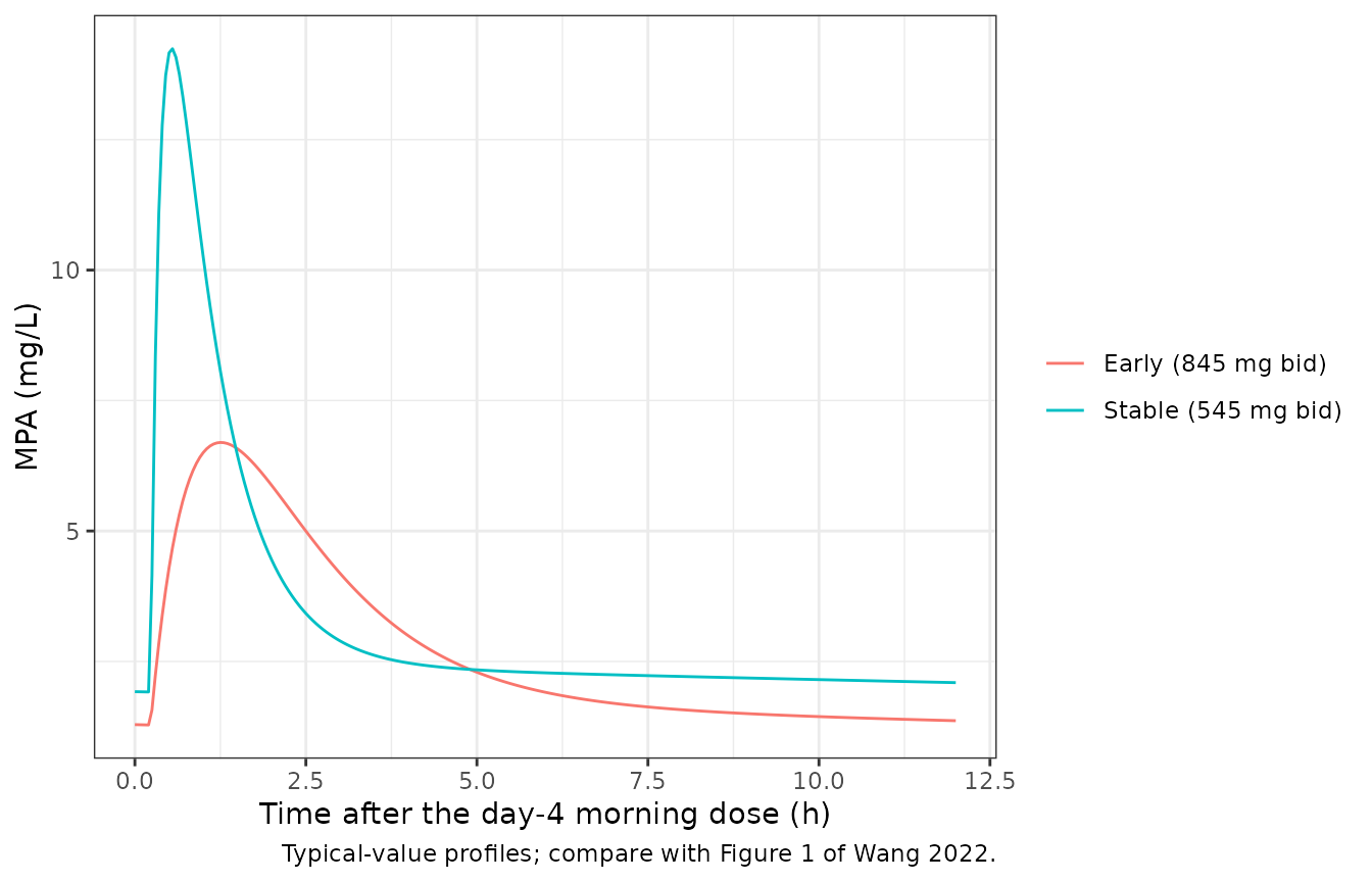
Virtual cohort and NCA against Table 2
Each stage gets 200 virtual patients. Per-subject daily MMF doses are drawn from a normal distribution with the Table 1 mean and SD for that stage, truncated to the Methods dose range (1.0-3.0 g/day early, 0.5-1.5 g/day stable) and given as two equal doses. The paper’s 10-point sampling schedule is simulated with residual error, as Table 2 is an NCA of observed concentrations: Cmax and Cmin are read directly from the sampled values and AUC0-12 uses the linear trapezoidal rule.
set.seed(20220509)
n_per_stage <- 200
draw_dose <- function(n, mean_day, sd_day, lo, hi) {
  d <- numeric(0)
  while (length(d) < n) {
    x <- stats::rnorm(n, mean_day, sd_day)
    d <- c(d, x[x >= lo & x <= hi])
  }
  d[seq_len(n)] / 2
}
cohort <- data.frame(
  id = seq_len(2 * n_per_stage),
  POSTTX_STABLE = rep(0:1, each = n_per_stage),
  dose = c(
    draw_dose(n_per_stage, 1690, 440, 1000, 3000),
    draw_dose(n_per_stage, 1090, 290, 500, 1500)
  )
)
ev_cohort <- make_events(cohort$id, cohort$dose, t_day4 + samp) |>
  dplyr::left_join(dplyr::select(cohort, id, POSTTX_STABLE), by = "id")

rxode2::rxSetSeed(20220509)
sim <- rxode2::rxSolve(mod, ev_cohort, returnType = "data.frame", maxsteps = 1e6) |>
  dplyr::select(-dplyr::any_of(c("POSTTX_STABLE", "dose"))) |>
  dplyr::left_join(cohort, by = "id") |>
  dplyr::mutate(treatment = ifelse(POSTTX_STABLE == 1, "Stable state", "Early stage"))
stopifnot(!anyNA(sim$sim), nrow(sim) == nrow(cohort) * length(samp))
sim |>
  dplyr::mutate(tad = time - t_day4) |>
  dplyr::group_by(treatment, tad) |>
  dplyr::summarise(
    p05 = quantile(sim, 0.05), p50 = median(sim), p95 = quantile(sim, 0.95),
    .groups = "drop"
  ) |>
  ggplot(aes(tad, p50)) +
  geom_ribbon(aes(ymin = p05, ymax = p95), alpha = 0.25) +
  geom_line() +
  facet_wrap(~treatment) +
  labs(
    x = "Time after dose (h)", y = "MPA (mg/L)",
    caption = "Simulated 5th-50th-95th percentiles with residual error; compare with Figure 4 of Wang 2022."
  ) +
  theme_bw()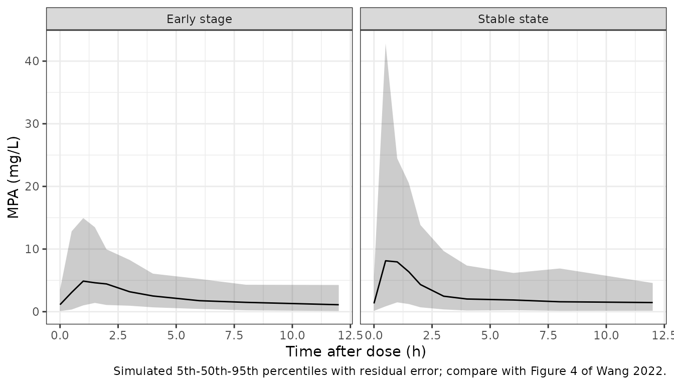
# Interval-relative time: the dose of the sampled interval is at time 0.
conc_df <- sim |>
  dplyr::transmute(id, treatment, time = time - t_day4, conc = sim) |>
  dplyr::filter(!is.na(conc))
# A normal proportional error makes Cc * (1 + eps) negative when eps < -1
# (P = 0.0035 for sd 0.37). Such samples would read as below the assay limit,
# so they enter the NCA as zero.
stopifnot(mean(conc_df$conc < 0) < 0.02)
conc_df$conc <- pmax(conc_df$conc, 0)
dose_df <- cohort |>
  dplyr::mutate(
    treatment = ifelse(POSTTX_STABLE == 1, "Stable state", "Early stage"),
    time = 0
  ) |>
  dplyr::select(id, treatment, time, dose)

intervals <- data.frame(
  start = 0, end = 12, cmax = TRUE, cmin = TRUE, tmax = TRUE, auclast = TRUE
)
run_nca <- function(trt) {
  o_conc <- PKNCA::PKNCAconc(dplyr::filter(conc_df, treatment == trt), conc ~ time | treatment + id)
  o_dose <- PKNCA::PKNCAdose(dplyr::filter(dose_df, treatment == trt), dose ~ time | treatment + id)
  o_data <- PKNCA::PKNCAdata(o_conc, o_dose,
    intervals = intervals,
    options = list(auc.method = "linear")
  )
  as.data.frame(PKNCA::pk.nca(o_data))
}
nca_res <- dplyr::bind_rows(lapply(unique(conc_df$treatment), run_nca))

# Table 2 reports arithmetic means, so aggregate to means before comparing.
sim_mean <- nca_res |>
  dplyr::filter(PPTESTCD %in% c("cmax", "cmin", "tmax", "auclast")) |>
  dplyr::group_by(treatment, PPTESTCD) |>
  dplyr::summarise(PPORRES = mean(PPORRES), .groups = "drop")

published <- data.frame(
  treatment = c("Early stage", "Stable state"),
  auclast = c(32.61, 42.30),
  cmax = c(9.83, 16.87),
  cmin = c(0.96, 1.29),
  # Table 2 Tmax is on the dataset clock (74.10 and 72.82 h); the sampled
  # interval starts at 72 h.
  tmax = c(74.10, 72.82) - 72
)
cmp <- nlmixr2lib::ncaComparisonTable(
  simulated = sim_mean,
  reference = published,
  by = "treatment",
  units = c(cmax = "mg/L", cmin = "mg/L", tmax = "h", auclast = "mg*h/L"),
  tolerance_pct = 20
)
knitr::kable(cmp,
  caption = paste(
    "Simulated (mean of 200 virtual patients per stage) vs Wang 2022 Table 2",
    "(mean of observed NCA). * differs from the reference by more than 20%."
  )
)| NCA parameter | treatment | Reference | Simulated | % diff |
|---|---|---|---|---|
| Cmax (mg/L) | Early stage | 9.83 | 8.36 | -15.0% |
| Cmax (mg/L) | Stable state | 16.9 | 16.6 | -1.5% |
| Cmin (mg/L) | Early stage | 0.96 | 0.811 | -15.5% |
| Cmin (mg/L) | Stable state | 1.29 | 1.01 | -22.0%* |
| Tmax (h) | Early stage | 2.1 | 1.71 | -18.5% |
| Tmax (h) | Stable state | 0.82 | 1.02 | +24.4%* |
| AUClast (mg*h/L) | Early stage | 32.6 | 32.9 | +0.8% |
| AUClast (mg*h/L) | Stable state | 42.3 | 42.9 | +1.5% |
attr(cmp, "footnote")
#> [1] "* differs from reference by more than ±20%."
get_sim <- function(trt, p) {
  v <- sim_mean$PPORRES[sim_mean$treatment == trt & sim_mean$PPTESTCD == p]
  if (length(v) != 1L) stop("no unique simulated value for ", trt, " / ", p)
  v
}
auc_pct <- c(
  100 * (get_sim("Early stage", "auclast") / 32.61 - 1),
  100 * (get_sim("Stable state", "auclast") / 42.30 - 1)
)
auc_ratio <- get_sim("Stable state", "auclast") / get_sim("Early stage", "auclast")
stopifnot(
  # AUC0-12 is dose / CL-dominated: a wrong clearance, stage effect or dose
  # unit moves it by tens of percent. The mean of 200 subjects with
  # omega^2(CL) = 0.20 has a Monte Carlo SE of about 3%.
  all(abs(auc_pct) < 15),
  # Table 2: 42.30 / 32.61 = 1.30 despite a 35% lower stable-state dose.
  abs(auc_ratio / (42.30 / 32.61) - 1) < 0.2
)
AUC0-12 is reproduced within a few percent in both stages, as is the stable-state Cmax. The early-stage Cmax runs about 15% below the observed mean and the early-stage Tmax is earlier than observed (2.1 h after the dose): ka and Tlag are shared by both stages, so the model cannot reproduce the slower early-stage absorption that the observed Tmax suggests, and the stable-state Tmax is correspondingly a little later than observed. Cmin is about 15-20% below the observed means in both stages. None of these move the AUC, which is the quantity the paper’s dosing recommendations rest on.
Monte Carlo dosing simulation (Figure 5)
Wang 2022 simulated six fixed regimens in each stage (0.25-1.5 g bid, 1000 virtual patients each) and reported the percentage of patients with a day-4 AUC0-12 in the 30-60 mg h/L target window. Here each arm has 200 virtual patients; AUC0-12 is integrated from the individual predictions on a 0.1-h grid.
regimens <- c(250, 500, 750, 1000, 1250, 1500)
n_pta <- 200
pta_design <- tidyr::expand_grid(POSTTX_STABLE = 0:1, dose = regimens) |>
  dplyr::mutate(arm = dplyr::row_number())
pta_cohort <- pta_design[rep(seq_len(nrow(pta_design)), each = n_pta), ] |>
  dplyr::mutate(id = dplyr::row_number())
ev_pta <- make_events(pta_cohort$id, pta_cohort$dose, t_day4 + seq(0, 12, by = 0.1)) |>
  dplyr::left_join(dplyr::select(pta_cohort, id, POSTTX_STABLE), by = "id")

rxode2::rxSetSeed(859351)
sim_pta <- rxode2::rxSolve(mod, ev_pta, returnType = "data.frame", maxsteps = 1e6)
stopifnot(!anyNA(sim_pta$Cc))
auc_pta <- sim_pta |>
  dplyr::group_by(id) |>
  dplyr::summarise(auc = trap(time, Cc), .groups = "drop") |>
  dplyr::left_join(pta_cohort, by = "id") |>
  dplyr::mutate(stage = ifelse(POSTTX_STABLE == 1, "Stable state", "Early stage"))

pta <- auc_pta |>
  dplyr::group_by(stage, dose) |>
  dplyr::summarise(simulated = 100 * mean(auc >= 30 & auc <= 60), .groups = "drop") |>
  dplyr::arrange(stage, dose) |>
  dplyr::mutate(
    # Results 'Model-Based Simulations'.
    published = c(0.1, 9.0, 41.2, 59.4, 62.0, 51.2, 7.3, 60.1, 53.3, 31.7, 15.0, 7.5),
    difference = simulated - published
  )
knitr::kable(
  dplyr::rename(pta,
    "Stage" = stage, "MMF dose (mg bid)" = dose,
    "Simulated in target (%)" = simulated, "Published in target (%)" = published,
    "Difference (points)" = difference
  ),
  digits = 1,
  caption = "Probability of a day-4 AUC0-12 of 30-60 mg h/L."
)| Stage | MMF dose (mg bid) | Simulated in target (%) | Published in target (%) | Difference (points) |
|---|---|---|---|---|
| Early stage | 250 | 0.5 | 0.1 | 0.4 |
| Early stage | 500 | 7.5 | 9.0 | -1.5 |
| Early stage | 750 | 37.5 | 41.2 | -3.7 |
| Early stage | 1000 | 59.0 | 59.4 | -0.4 |
| Early stage | 1250 | 58.5 | 62.0 | -3.5 |
| Early stage | 1500 | 50.5 | 51.2 | -0.7 |
| Stable state | 250 | 9.5 | 7.3 | 2.2 |
| Stable state | 500 | 47.0 | 60.1 | -13.1 |
| Stable state | 750 | 50.0 | 53.3 | -3.3 |
| Stable state | 1000 | 28.5 | 31.7 | -3.2 |
| Stable state | 1250 | 24.5 | 15.0 | 9.5 |
| Stable state | 1500 | 13.0 | 7.5 | 5.5 |
auc_pta |>
  ggplot(aes(factor(dose / 1000), auc)) +
  geom_boxplot(outlier.size = 0.5) +
  geom_hline(yintercept = c(30, 60), linetype = "dashed", colour = "red") +
  facet_wrap(~stage) +
  labs(
    x = "MMF dose (g bid)", y = "Day-4 AUC0-12 (mg h/L)",
    caption = "Replicates Figure 5 of Wang 2022."
  ) +
  theme_bw()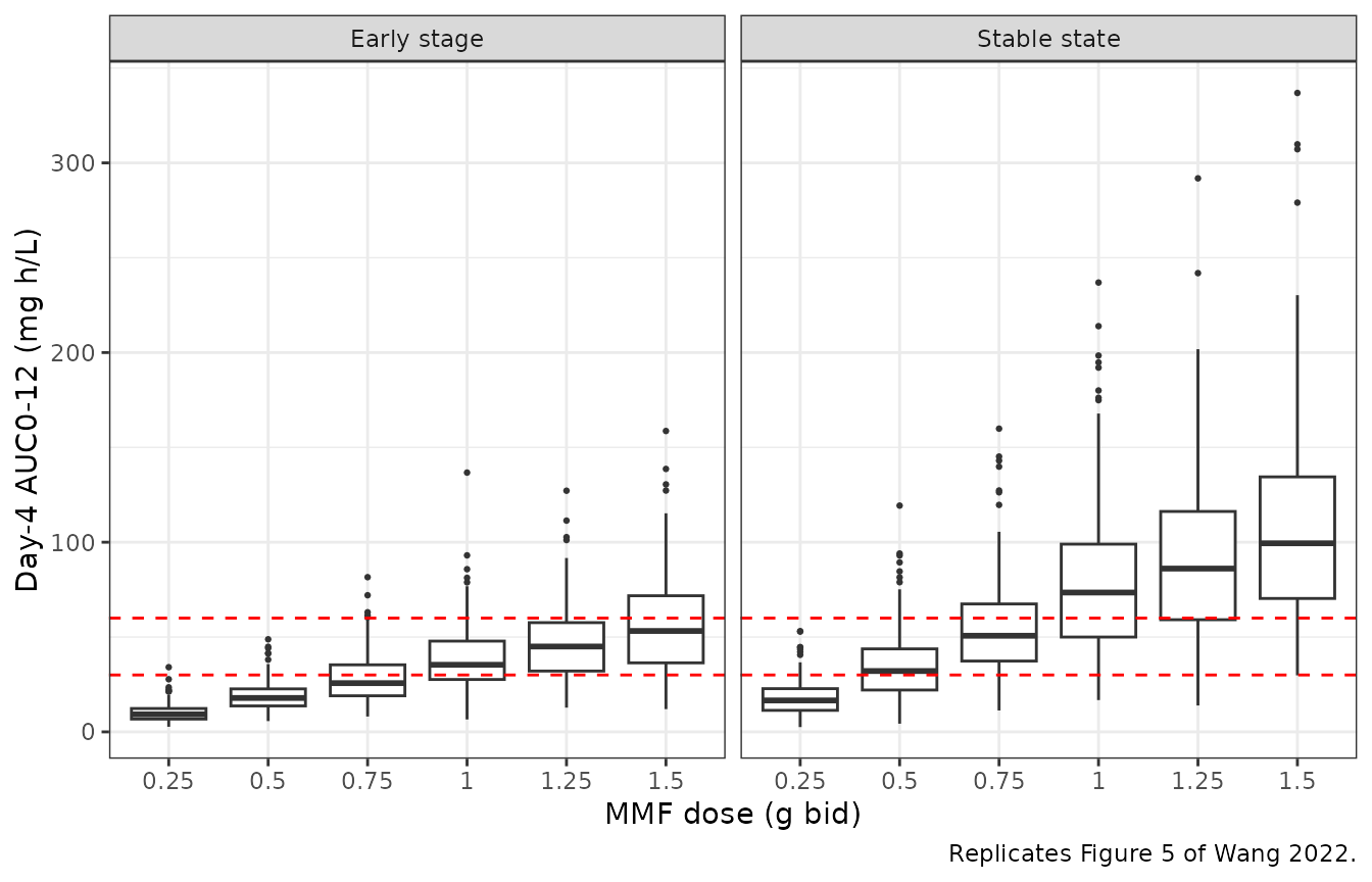
best <- pta |>
  dplyr::group_by(stage) |>
  dplyr::slice_max(simulated, n = 1, with_ties = FALSE)
pta_cell <- function(stg, d) {
  v <- pta$simulated[pta$stage == stg & pta$dose == d]
  if (length(v) != 1L) stop("no unique PTA cell for ", stg, " at ", d, " mg")
  v
}
mad_stage <- tapply(abs(pta$difference), pta$stage, mean)
stopifnot(
  nrow(pta) == 12L,
  # Binomial SE of one 200-subject cell is <= 3.5 points. Mean absolute
  # differences were 2.4 / 5.3 points (early / stable) in a 1000-subject run
  # by the maintainers and 1.7 / 6.1 in this cohort; a mis-transcribed CL,
  # stage effect or dose unit shifts whole columns by tens of points.
  all(mad_stage < 10),
  # The paper's recommendation: 1.0-1.5 g bid early, 0.50-0.75 g bid stable.
  best$dose[best$stage == "Early stage"] %in% c(1000, 1250, 1500),
  best$dose[best$stage == "Stable state"] %in% c(500, 750),
  # Crossing of the two stages: tens of points apart at both ends.
  pta_cell("Stable state", 500) - pta_cell("Early stage", 500) > 25,
  pta_cell("Early stage", 1250) - pta_cell("Stable state", 1250) > 20
)
mad_stage
#>  Early stage Stable state
#>     1.700000     6.133333
The simulated target-attainment pattern reproduces the paper’s: the early stage needs 1.0-1.5 g bid and the stable state 0.50-0.75 g bid. The early stage matches cell by cell. In the stable state the 0.5 g bid arm attains the target somewhat less often than published and the 1.25-1.5 g bid arms somewhat more often, i.e. the simulated stable-state AUC distribution is a little wider than the paper’s; the same pattern appeared in a 1000-patient run by the maintainers (52% at 0.5 g bid, 22% at 1.25 g bid), so it is not only Monte Carlo noise. The paper does not describe its simulation settings beyond the regimens and the cohort size.
Assumptions and deviations
-
Stable-state V/F. The Abstract and Results quote a
stable-state V/F of 16.24 L, but Table 3’s
dVdStage = -2.54with the exponential form that reproduces the quoted stable CL/F (10.25 L/h) gives 78.07 x exp(-2.54) = 6.16 L. The coefficient is internally consistent with its own uncertainty (CV 15.32%, 95% CI -3.29 to -1.77) and bootstrap median (-2.36), and no other parameterisation reproduces 16.24 L (log(16.24 / 78.07) = -1.57 lies outside the CI). The model therefore encodes Table 3. A simulation by the maintainers at the stable-state mean dose gave a mean steady-state Cmax of about 15 mg/L with -2.54 versus about 11 mg/L with V/F = 16.24 L, against an observed Table 2 Cmax of 16.87 mg/L, which also favours Table 3. AUC is unaffected by the choice. - Doses are mg of MMF. The model has no MMF-to-MPA molecular-weight conversion: Table 2’s NCA CL/F equals MMF dose / AUC, and the simulated AUC0-12 reproduces Table 2 with the dose entered as mg MMF. All apparent clearances and volumes are relative to the MMF dose.
-
Post-transplant stage covariate.
POSTTX_STABLEis the paper’s own binaryStagecolumn (0 = early, 1 = stable). The cohort contains only patients sampled on days 4-8 or after 5.5-10 years, so the model says nothing about intermediate post-transplant times and no day-count threshold is implied. - No IIV covariances. Table 3 reports only diagonal variances; the matrix is diagonal.
- Virtual cohort. Per-subject doses are drawn from a truncated normal distribution built from Table 1’s mean and SD; the paper does not give the dose distribution. No other covariate enters the model.
- Day-4 sampling. Table 2’s Tmax values (74.10 and 72.82 h) indicate that the sampled interval starts at 72 h, matching the Methods statement that sampling was at least 3 days after the same dose and the Monte Carlo simulations’ “AUCss,12h on day 4”. The NCA and PTA simulations use seven doses at 0-72 h and sample 72-84 h.
- Monte Carlo details. The paper does not say whether its simulated AUCs included residual error; the PTA here uses individual predictions without residual error, which reproduces the published percentages closely.
- Supplement. Supplementary Tables S1-S2 and Figures S1-S2 (the enterohepatic-circulation model comparison, covariate screening and limited-sampling regression equations) are not needed for the final model, whose parameters are all in Table 3. No erratum was found in a literature check on 2026-10-02.