Calcitriol-conjugated quantum dots in mice with inflammatory breast cancer (Forder 2019)

Model and source

• Citation: Forder J, Smith M, Wagner M, Schaefer RJ, Gorky J, van Golen KL, Nohe A, Dhurjati P (2019). A physiologically-based pharmacokinetic model for targeting calcitriol-conjugated quantum dots to inflammatory breast cancer cells. Clin Transl Sci 12(6):617-624.
• Article: https://doi.org/10.1111/cts.12664 (open access, PMC6853145)
• Supplement: Figures S1-S3, Tables S1-S2 and the authors’ complete MATLAB model code (CTS-12-617-s006.docx), from the EuropePMC supplementary-file bundle for PMC6853145.

Forder 2019 builds a small flow-limited PBPK model for the distribution of fluorescent quantum dots (QDs) after one intravenous injection in mice. Three QDs are modelled: unconjugated control QDs (ConQD), calcitriol-conjugated QDs (CalQD), and CalQDs that also carry the SM3 anti-MUC1 antibody (SM3 CalQD), which targets inflammatory breast cancer (IBC) cells. There are three connectivities (Figure 1): a healthy (tumor-free) mouse, an early-stage IBC mouse with a tumor inside breast tissue, and a late-stage IBC mouse with metastatic tumor tissue in parallel with the other organs. The authors fitted the partition coefficients separately for each of the 3 x 3 combinations, so the package has nine models:

qds <- c(
  ConQD = "controlQuantumDot",
  CalQD = "calcitriolQuantumDot",
  "SM3 CalQD" = "sm3CalcitriolQuantumDot"
)
stages <- c(Healthy = "healthy", "Early-stage" = "earlyIBC", "Late-stage" = "lateIBC")
grid <- expand.grid(qd = names(qds), stage = names(stages), stringsAsFactors = FALSE)
grid$model <- sprintf("Forder_2019_%s_%s_mouse_pbpk", qds[grid$qd], stages[grid$stage])
stopifnot(all(grid$model %in% modeldb$name))
knitr::kable(grid |> rename(QD = qd, Stage = stage, Model = model))

QD	Stage	Model
ConQD	Healthy	Forder_2019_controlQuantumDot_healthy_mouse_pbpk
CalQD	Healthy	Forder_2019_calcitriolQuantumDot_healthy_mouse_pbpk
SM3 CalQD	Healthy	Forder_2019_sm3CalcitriolQuantumDot_healthy_mouse_pbpk
ConQD	Early-stage	Forder_2019_controlQuantumDot_earlyIBC_mouse_pbpk
CalQD	Early-stage	Forder_2019_calcitriolQuantumDot_earlyIBC_mouse_pbpk
SM3 CalQD	Early-stage	Forder_2019_sm3CalcitriolQuantumDot_earlyIBC_mouse_pbpk
ConQD	Late-stage	Forder_2019_controlQuantumDot_lateIBC_mouse_pbpk
CalQD	Late-stage	Forder_2019_calcitriolQuantumDot_lateIBC_mouse_pbpk
SM3 CalQD	Late-stage	Forder_2019_sm3CalcitriolQuantumDot_lateIBC_mouse_pbpk

Population

ui_sm3_late <- rxode2::rxode(readModelDb("Forder_2019_sm3CalcitriolQuantumDot_lateIBC_mouse_pbpk"))
str(ui_sm3_late$population)
#> List of 9
#>  $ species       : chr "mouse (female, 13-16 weeks, ~22 g)"
#>  $ n_subjects    : int NA
#>  $ n_studies     : int 1
#>  $ age_range     : chr "13-16 weeks"
#>  $ weight_range  : chr "~22.0 g (fixed model body weight)"
#>  $ sex_female_pct: num 100
#>  $ disease_state : chr "late-stage (metastatic) inflammatory breast cancer (SUM149 xenograft)"
#>  $ dose_range    : chr "Single intravenous injection of SM3 CalQD; the model code starts plasma at 40 nM (43.12 pmol in 1.078 mL)."
#>  $ notes         : chr "Partition coefficients were fitted (MATLAB fmincon, relative squared error) to mean day-4 (96 h) fluorescence p"| __truncated__

The biodistribution data are from Schaefer 2012 (reference 10 of the paper): female mice aged 13-16 weeks (about 22.0 g), with or without SUM149 IBC tumors, imaged by fluorescence 4 days after injection. Only the mean pixel intensity per organ (Table 2) was used, and there are no early-stage data, so the early-stage partition coefficients were fitted to the late-stage intensities. The number of animals is not reported. No between-subject variability or residual error was estimated, so every model here is a deterministic typical-value model.

Source trace

Item	Source	Notes
Organ volumes v_*	Table 1; supplementary code vp, vk, …	Code values (more digits) used, e.g. v_liver 1.2078 vs Table 1 1.208
Organ plasma flows q_*	Table 1; supplementary code qk, qli, …	See the q_other note under Errata
v_spleen enlarged 0.154 mL	Table 1 (parenthesis)	Used only in the Figure 3 / Table S2 section below
kelim = 1e-6	Eq. 3; code k1 = 0.000001	Sits inside the 1/V_liver bracket of Eq. 12
lkp_other = log(1)	Results, Partition coefficients; code ro = 1	Assumed, not fitted
lkp_kidney, lkp_liver, lkp_spleen, lkp_lung	Table 3	One column per QD x stage
lkp_tumor	Table 3	Early- and late-stage models only
lkp_breast	Table 3	Early-stage models only
Organ ODE dC/dt = Q/V (C_p - C/P)	Eq. 6, 9-11, 13, 16
Liver ODE (spleen outflow + hepatic artery in, elimination)	Eq. 12
Healthy plasma ODE	Eq. 7-8	Identical to the code
Late-stage plasma ODE	Supplementary code Tsm3QD_MW()	Differs from printed Eq. 14; see Errata
Early-stage plasma, breast and tumor ODEs	Eq. 17-18; code Tsm3QD()	Breast/tumor coupling differs from printed Eq. 19-20; see Errata
IV pulse into plasma; 40 nM initial plasma concentration	Methods; code ode23s(..., [40; 0; ...])	Dose here: 40 nM x 1.078 mL = 43.12 pmol
Fit target: organ intensities at 96 h	Table 2; code TSoS() / nTSoS() / Tsm3QDSoS()
Enlarged-spleen partition coefficients	Table S2	Section “Enlarged spleen”

Simulation set-up

Every model is dosed with the code’s 40 nM initial plasma concentration (43.12 pmol into plasma). Observation rows are placed on the plasma ODE state, and all organ concentrations are returned alongside because each state already holds a concentration.

dose_pmol <- 40 * 1.078
times <- sort(unique(c(seq(0, 12, by = 0.02), seq(12, 96, by = 0.25))))

make_events <- function(times) {
  rxode2::et(amt = dose_pmol, cmt = "plasma") |>
    rxode2::et(times, cmt = "plasma")
}

sim_model <- function(name, times, ...) {
  ui <- rxode2::rxode(readModelDb(name))
  out <- rxode2::rxSolve(ui, make_events(times), returnType = "data.frame", ...)
  if (is.null(out$id)) out$id <- 1L
  out$model <- name
  out
}

sims <- lapply(grid$model, sim_model, times = times)
names(sims) <- grid$model

Reproducing the fit: Table 3 partition coefficients against Table 2

Table 3 reports the partition coefficients that minimise the relative squared error between simulated and observed day-4 (96 h) intensities for kidney, liver, spleen and lung. Simulating each packaged model to 96 h and comparing against Table 2 therefore checks the whole transcription (topology, volumes, flows, partition coefficients, dose) at once. There is no residual error or between-subject variability, so this is a deterministic check and a tight tolerance is appropriate.

table2 <- tibble::tribble(
  ~qd, ~data, ~kidney, ~liver, ~lung, ~spleen,
  "ConQD", "No tumor", 10.40, 16.23, 4.66, 12.73,
  "CalQD", "No tumor", 11.01, 20.38, 3.16, 10.99,
  "SM3 CalQD", "No tumor", 10.47, 17.18, 5.01, 9.87,
  "ConQD", "Late-stage tumor", 12.54, 14.85, 8.22, 26.43,
  "CalQD", "Late-stage tumor", 15.15, 20.15, 7.59, 21.46,
  "SM3 CalQD", "Late-stage tumor", 11.57, 18.12, 7.46, 17.92
) |>
  pivot_longer(c(kidney, liver, lung, spleen), names_to = "organ", values_to = "observed")

day4 <- bind_rows(sims) |>
  filter(abs(time - 96) < 1e-8) |>
  select(model, kidney, liver, lung, spleen) |>
  left_join(grid, by = "model") |>
  pivot_longer(c(kidney, liver, lung, spleen), names_to = "organ", values_to = "simulated") |>
  mutate(data = ifelse(stage == "Healthy", "No tumor", "Late-stage tumor")) |>
  left_join(table2, by = c("qd", "data", "organ")) |>
  mutate(pct_diff = 100 * (simulated - observed) / observed)

stopifnot(nrow(day4) == 36, !anyNA(day4$pct_diff))

day4 |>
  mutate(simulated = signif(simulated, 4), pct_diff = round(pct_diff, 2)) |>
  select(stage, qd, organ, observed, simulated, pct_diff) |>
  rename(
    Stage = stage, QD = qd, Organ = organ,
    "Table 2 intensity" = observed, "Simulated at 96 h" = simulated,
    "Difference (%)" = pct_diff
  ) |>
  knitr::kable()

Stage	QD	Organ	Table 2 intensity	Simulated at 96 h	Difference (%)
Healthy	ConQD	kidney	10.40	10.390	-0.13
Healthy	ConQD	liver	16.23	16.170	-0.39
Healthy	ConQD	lung	4.66	4.637	-0.49
Healthy	ConQD	spleen	12.73	12.710	-0.20
Healthy	CalQD	kidney	11.01	10.990	-0.21
Healthy	CalQD	liver	20.38	20.220	-0.80
Healthy	CalQD	lung	3.16	3.139	-0.66
Healthy	CalQD	spleen	10.99	10.990	-0.03
Healthy	SM3 CalQD	kidney	10.47	10.460	-0.07
Healthy	SM3 CalQD	liver	17.18	17.080	-0.60
Healthy	SM3 CalQD	lung	5.01	4.991	-0.38
Healthy	SM3 CalQD	spleen	9.87	9.861	-0.09
Early-stage	ConQD	kidney	12.54	12.540	0.01
Early-stage	ConQD	liver	14.85	14.850	-0.01
Early-stage	ConQD	lung	8.22	8.231	0.13
Early-stage	ConQD	spleen	26.43	26.420	-0.05
Early-stage	CalQD	kidney	15.15	15.160	0.05
Early-stage	CalQD	liver	20.15	20.140	-0.04
Early-stage	CalQD	lung	7.59	7.595	0.07
Early-stage	CalQD	spleen	21.46	21.460	-0.02
Early-stage	SM3 CalQD	kidney	11.57	11.950	3.27
Early-stage	SM3 CalQD	liver	18.12	18.720	3.32
Early-stage	SM3 CalQD	lung	7.46	7.703	3.26
Early-stage	SM3 CalQD	spleen	17.92	18.500	3.23
Late-stage	ConQD	kidney	12.54	12.540	0.00
Late-stage	ConQD	liver	14.85	14.820	-0.17
Late-stage	ConQD	lung	8.22	8.209	-0.13
Late-stage	ConQD	spleen	26.43	26.460	0.12
Late-stage	CalQD	kidney	15.15	15.140	-0.08
Late-stage	CalQD	liver	20.15	20.080	-0.34
Late-stage	CalQD	lung	7.59	7.579	-0.14
Late-stage	CalQD	spleen	21.46	21.450	-0.05
Late-stage	SM3 CalQD	kidney	11.57	11.540	-0.24
Late-stage	SM3 CalQD	liver	18.12	18.030	-0.49
Late-stage	SM3 CalQD	lung	7.46	7.455	-0.06
Late-stage	SM3 CalQD	spleen	17.92	17.910	-0.07

max_err <- day4 |>
  group_by(stage, qd) |>
  summarise(max_abs_pct = max(abs(pct_diff)), .groups = "drop")
knitr::kable(max_err |> rename(Stage = stage, QD = qd, "Max abs difference (%)" = max_abs_pct), digits = 2)

Stage	QD	Max abs difference (%)
Early-stage	CalQD	0.07
Early-stage	ConQD	0.13
Early-stage	SM3 CalQD	3.32
Healthy	CalQD	0.80
Healthy	ConQD	0.49
Healthy	SM3 CalQD	0.60
Late-stage	CalQD	0.34
Late-stage	ConQD	0.17
Late-stage	SM3 CalQD	0.49

is_sm3_early <- max_err$stage == "Early-stage" & max_err$qd == "SM3 CalQD"
stopifnot(
  # Eight of nine fits reproduce Table 2 to rounding of the printed
  # partition coefficients.
  all(max_err$max_abs_pct[!is_sm3_early] < 1.5),
  # The early-stage SM3 CalQD column does not (see Errata): it over-predicts
  # every organ by about 3 percent.
  max_err$max_abs_pct[is_sm3_early] > 2.5,
  max_err$max_abs_pct[is_sm3_early] < 4
)

Eight of the nine models reproduce the fitted intensities to within the rounding of the printed partition coefficients. The early-stage SM3 CalQD model over-predicts every organ by about 3%; the reason is shown in the next section.

Enlarged spleen (Table S2)

The authors also refitted the tumor models with the spleen volume doubled to 0.154 mL (splenomegaly), keeping the spleen blood flow (Table S2). These fits are a sensitivity analysis and are not shipped as separate models; they are reproduced here by overriding v_spleen and the partition coefficients in the packaged early- and late-stage models.

tableS2 <- tibble::tribble(
  ~stage, ~qd, ~kidney, ~liver, ~spleen, ~lung, ~tumor, ~breast,
  "Early-stage", "ConQD", 51.6, 61.1, 109, 33.8, 33.5, 2.8,
  "Early-stage", "CalQD", 113, 151, 160, 56.7, 63.4, 2.9,
  "Early-stage", "SM3 CalQD", 59.1, 92.6, 91.5, 38.1, 97.4, 1.83,
  "Late-stage", "ConQD", 53.8, 63.6, 113, 35.2, 33.5, NA,
  "Late-stage", "CalQD", 103, 136, 145, 51.4, 45.7, NA,
  "Late-stage", "SM3 CalQD", 55.6, 86.7, 86.1, 35.8, 97.5, NA
)

sim_enlarged <- function(i) {
  r <- tableS2[i, ]
  name <- grid$model[grid$qd == r$qd & grid$stage == r$stage]
  kp <- c(kidney = r$kidney, liver = r$liver, spleen = r$spleen, lung = r$lung, tumor = r$tumor)
  if (!is.na(r$breast)) kp <- c(kp, breast = r$breast)
  params <- c(v_spleen = 0.154, stats::setNames(log(kp), paste0("lkp_", names(kp))))
  ui <- rxode2::rxode(readModelDb(name))
  ui <- suppressMessages(do.call(rxode2::ini, c(list(ui), as.list(params))))
  out <- rxode2::rxSolve(ui, make_events(times), returnType = "data.frame")
  out$stage <- r$stage
  out$qd <- r$qd
  out
}
enlarged <- bind_rows(lapply(seq_len(nrow(tableS2)), sim_enlarged))

s2_check <- enlarged |>
  filter(abs(time - 96) < 1e-8) |>
  select(stage, qd, kidney, liver, lung, spleen) |>
  pivot_longer(c(kidney, liver, lung, spleen), names_to = "organ", values_to = "simulated") |>
  mutate(data = "Late-stage tumor") |>
  left_join(table2, by = c("qd", "data", "organ")) |>
  mutate(pct_diff = 100 * (simulated - observed) / observed)

stopifnot(nrow(s2_check) == 24, !anyNA(s2_check$pct_diff))
knitr::kable(
  s2_check |>
    group_by(stage, qd) |>
    summarise(max_abs_pct = max(abs(pct_diff)), .groups = "drop") |>
    rename(Stage = stage, QD = qd, "Max abs difference vs Table 2 (%)" = max_abs_pct),
  digits = 2
)

Stage	QD	Max abs difference vs Table 2 (%)
Early-stage	CalQD	0.35
Early-stage	ConQD	0.23
Early-stage	SM3 CalQD	0.07
Late-stage	CalQD	0.45
Late-stage	ConQD	0.27
Late-stage	SM3 CalQD	0.52

stopifnot(max(abs(s2_check$pct_diff)) < 1.5)

# The early-stage SM3 CalQD column of Table 3 is identical to its Table S2
# (enlarged-spleen) column; no other Table 3 / Table S2 pair coincides.
sm3_early_t3 <- rxode2::rxode(readModelDb(
  "Forder_2019_sm3CalcitriolQuantumDot_earlyIBC_mouse_pbpk"
))$theta[paste0("lkp_", c("kidney", "liver", "spleen", "lung", "tumor", "breast"))]
sm3_early_s2 <- unlist(tableS2[tableS2$stage == "Early-stage" & tableS2$qd == "SM3 CalQD", 3:8])
stopifnot(isTRUE(all.equal(unname(exp(sm3_early_t3)), unname(sm3_early_s2))))

All six enlarged-spleen fits reproduce Table 2 to rounding. The early-stage SM3 CalQD partition coefficients printed in Table 3 are exactly the Table S2 enlarged-spleen values. With the doubled spleen volume they fit Table 2 exactly. With the regular spleen volume, which is what Table 3 should describe, they are about 3% off. The regular-spleen fit for this QD therefore seems to have been replaced by the enlarged-spleen fit when the table was put together. The packaged model keeps the printed values (see Errata).

Mass balance

Elimination is negligible (kelim = 1e-6), so the total QD mass sum(V_i * C_i) should stay at the 43.12 pmol dose over 4 days.

vol_of <- function(name) {
  th <- rxode2::rxode(readModelDb(name))$theta
  th[grepl("^v_", names(th))]
}
mass <- bind_rows(lapply(grid$model, function(name) {
  v <- vol_of(name)
  s <- sims[[name]]
  organs <- sub("^v_", "", names(v))
  data.frame(
    model = name, time = s$time,
    mass = as.vector(as.matrix(s[, organs]) %*% v)
  )
})) |>
  left_join(grid, by = "model")

mass_summary <- mass |>
  group_by(stage, qd) |>
  summarise(
    max_mass = max(mass), mass_96h = mass[which.min(abs(time - 96))],
    .groups = "drop"
  ) |>
  mutate(pct_gain_96h = 100 * (mass_96h - dose_pmol) / dose_pmol)
knitr::kable(
  mass_summary |>
    rename(
      Stage = stage, QD = qd, "Max total (pmol)" = max_mass,
      "Total at 96 h (pmol)" = mass_96h, "Gain at 96 h (%)" = pct_gain_96h
    ),
  digits = 3
)

Stage	QD	Max total (pmol)	Total at 96 h (pmol)	Gain at 96 h (%)
Early-stage	CalQD	43.120	43.118	-0.004
Early-stage	ConQD	43.120	43.119	-0.003
Early-stage	SM3 CalQD	43.120	43.118	-0.004
Healthy	CalQD	43.120	43.118	-0.004
Healthy	ConQD	43.120	43.118	-0.004
Healthy	SM3 CalQD	43.120	43.118	-0.004
Late-stage	CalQD	44.688	44.685	3.629
Late-stage	ConQD	43.561	43.559	1.017
Late-stage	SM3 CalQD	44.659	44.616	3.470

late <- mass_summary$stage == "Late-stage"
stopifnot(
  # Healthy and early-stage topologies conserve mass exactly.
  all(abs(mass_summary$pct_gain_96h[!late]) < 0.01),
  # The late-stage plasma equation of the authors' code (used here) creates
  # a few percent of spurious mass; see Errata.
  all(mass_summary$pct_gain_96h[late] > 0.5),
  all(mass_summary$pct_gain_96h[late] < 4)
)

For comparison, here is the late-stage SM3 CalQD model with the printed Eq. 14 plasma equation, which returns (q_liver + q_spleen) * liver / kp_liver exactly as the healthy model does:

ui_late <- rxode2::rxode(readModelDb("Forder_2019_sm3CalcitriolQuantumDot_lateIBC_mouse_pbpk"))
ui_eq14 <- rxode2::model(
  ui_late,
  d / dt(plasma) <- (q_kidney * kidney / kp_kidney +
    (q_liver + q_spleen) * liver / kp_liver +
    q_lung * lung / kp_lung +
    q_other * other / kp_other +
    q_tumor * tumor / kp_tumor -
    q_total * plasma) / v_plasma
)
eq14 <- rxode2::rxSolve(ui_eq14, make_events(c(0, 96)), returnType = "data.frame")
eq14_96 <- eq14[eq14$time == 96, c("kidney", "liver", "lung", "spleen")]
obs_sm3_late <- table2$observed[table2$qd == "SM3 CalQD" & table2$data == "Late-stage tumor"]
eq14_pct <- 100 * (unlist(eq14_96) - obs_sm3_late) / obs_sm3_late
round(eq14_pct, 2)
#> kidney  liver   lung spleen 
#>  -3.59  -3.83  -3.42  -3.42
stopifnot(all(eq14_pct < -3), all(eq14_pct > -4.5))

The mass-conserving printed equation under-predicts all four Table 2 intensities by about 3.5% with the Table 3 partition coefficients. The code form matches them to rounding, which shows the Table 3 values were fitted with the code.

Replicating Figure 2 (SM3 CalQD, regular spleen)

Figure 2 plots each compartment’s concentration divided by the initial plasma concentration (40 nM). The healthy panel runs to 4 h and the tumor panels to 12 h.

norm <- function(df) {
  df |>
    select(time, plasma, kidney, liver, spleen, lung, other, any_of(c("tumor", "breast"))) |>
    pivot_longer(-time, names_to = "compartment", values_to = "conc") |>
    mutate(rel = conc / 40)
}
fig2 <- bind_rows(lapply(names(stages), function(st) {
  name <- grid$model[grid$qd == "SM3 CalQD" & grid$stage == st]
  tmax <- if (st == "Healthy") 4 else 12
  norm(sims[[name]]) |>
    filter(time <= tmax, compartment != "plasma", compartment != "other") |>
    mutate(stage = factor(st, levels = names(stages)))
}))
ggplot(fig2, aes(time, rel, colour = compartment)) +
  geom_line() +
  facet_wrap(~stage, scales = "free_x") +
  labs(
    x = "Time (hours)", y = "Relative concentration (C / C_plasma,0)",
    colour = NULL,
    caption = "Replicates Figure 2 of Forder 2019."
  ) +
  theme_bw()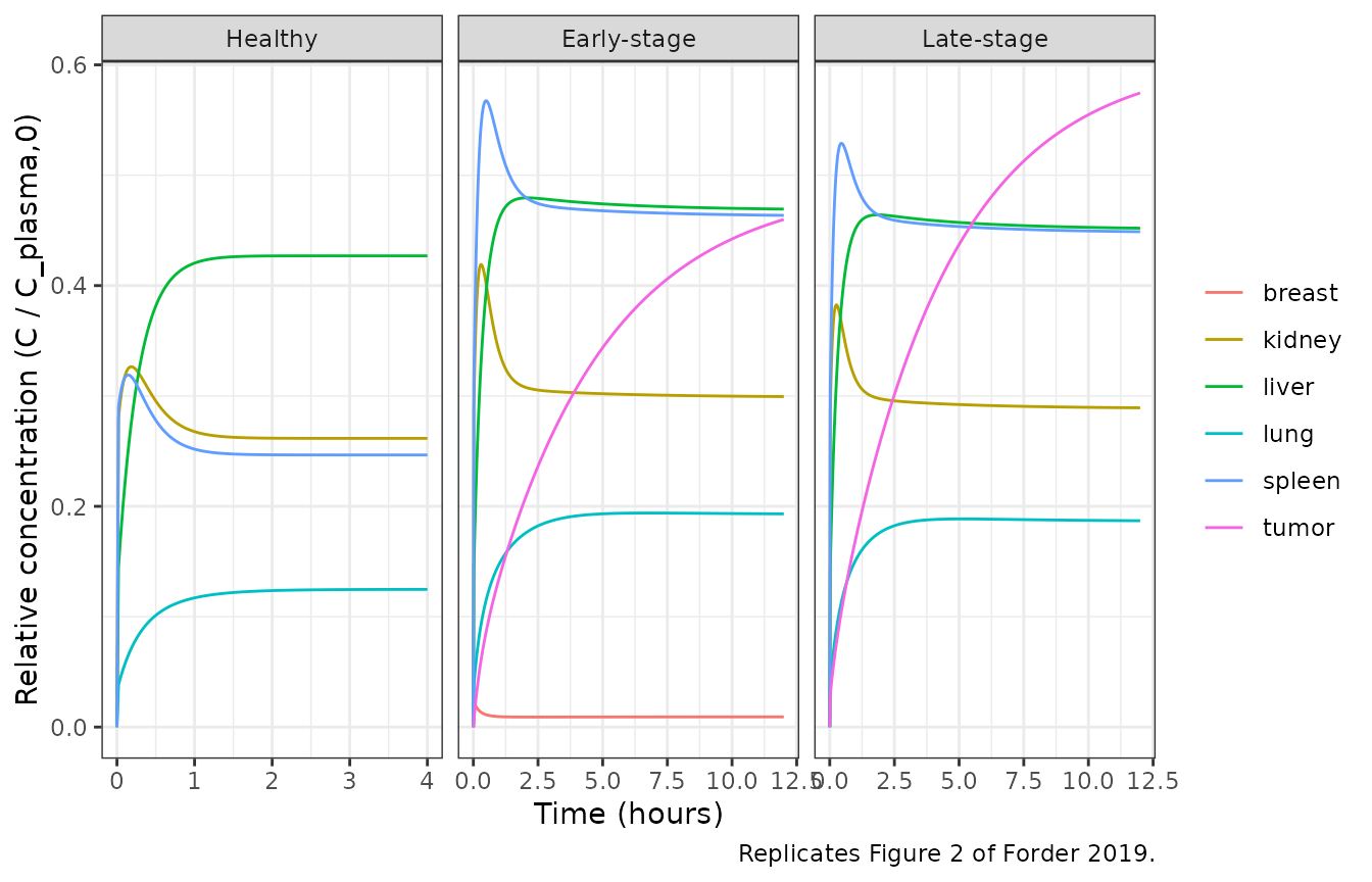

Figure 2 is described in the Results as follows. Spleen and kidney peak quickly and then redistribute, the other tissues rise monotonically, the tumor fills more slowly because its plasma flow is small, and in the early-stage model the breast stays low relative to the tumor. The quantitative claim is that the maximum SM3 CalQD tumor concentration is about 20% higher in the late-stage model than in the early-stage model.

tmax_of <- function(df, col) df$time[which.max(df[[col]])]
sm3 <- function(st) sims[[grid$model[grid$qd == "SM3 CalQD" & grid$stage == st]]]
claims <- tibble::tibble(
  stage = names(stages),
  spleen_tmax_h = vapply(names(stages), function(st) tmax_of(sm3(st), "spleen"), numeric(1)),
  kidney_tmax_h = vapply(names(stages), function(st) tmax_of(sm3(st), "kidney"), numeric(1)),
  tumor_cmax_nM = vapply(names(stages), function(st) {
    s <- sm3(st)
    if (is.null(s$tumor)) NA_real_ else max(s$tumor)
  }, numeric(1))
)
knitr::kable(
  claims |>
    rename(
      Stage = stage, "Spleen Tmax (h)" = spleen_tmax_h,
      "Kidney Tmax (h)" = kidney_tmax_h, "Tumor Cmax, 0-96 h (nM)" = tumor_cmax_nM
    ),
  digits = 3
)

Stage	Spleen Tmax (h)	Kidney Tmax (h)	Tumor Cmax, 0-96 h (nM)
Healthy	0.14	0.18	NA
Early-stage	0.50	0.30	19.692
Late-stage	0.46	0.26	24.298

tumor_ratio <- claims$tumor_cmax_nM[3] / claims$tumor_cmax_nM[2]
tumor_ratio
#> Late-stage 
#>   1.233889
stopifnot(
  # Spleen and kidney peak within the first hour.
  all(claims$spleen_tmax_h < 1), all(claims$kidney_tmax_h < 1),
  # Paper: late-stage tumor Cmax ~20% higher than early-stage (1.23 here).
  tumor_ratio > 1.15, tumor_ratio < 1.3
)

The simulated late-to-early tumor Cmax ratio is 1.23, consistent with the paper’s “~20% higher”. The early-stage value uses the Table 3 SM3 CalQD partition coefficients discussed under Errata.

Replicating Figure 3 (late-stage spleen, regular vs enlarged)

fig3 <- bind_rows(
  bind_rows(lapply(names(qds), function(q) {
    sims[[grid$model[grid$qd == q & grid$stage == "Late-stage"]]] |>
      mutate(qd = q, spleen_size = "Regular")
  })),
  enlarged |> filter(stage == "Late-stage") |> mutate(spleen_size = "Enlarged")
) |>
  filter(time <= 12)
ggplot(fig3, aes(time, spleen / 40, colour = qd, linetype = spleen_size)) +
  geom_line() +
  labs(
    x = "Time (hours)", y = "Relative spleen concentration",
    colour = NULL, linetype = "Spleen",
    caption = "Replicates Figure 3 of Forder 2019 (late-stage model)."
  ) +
  theme_bw()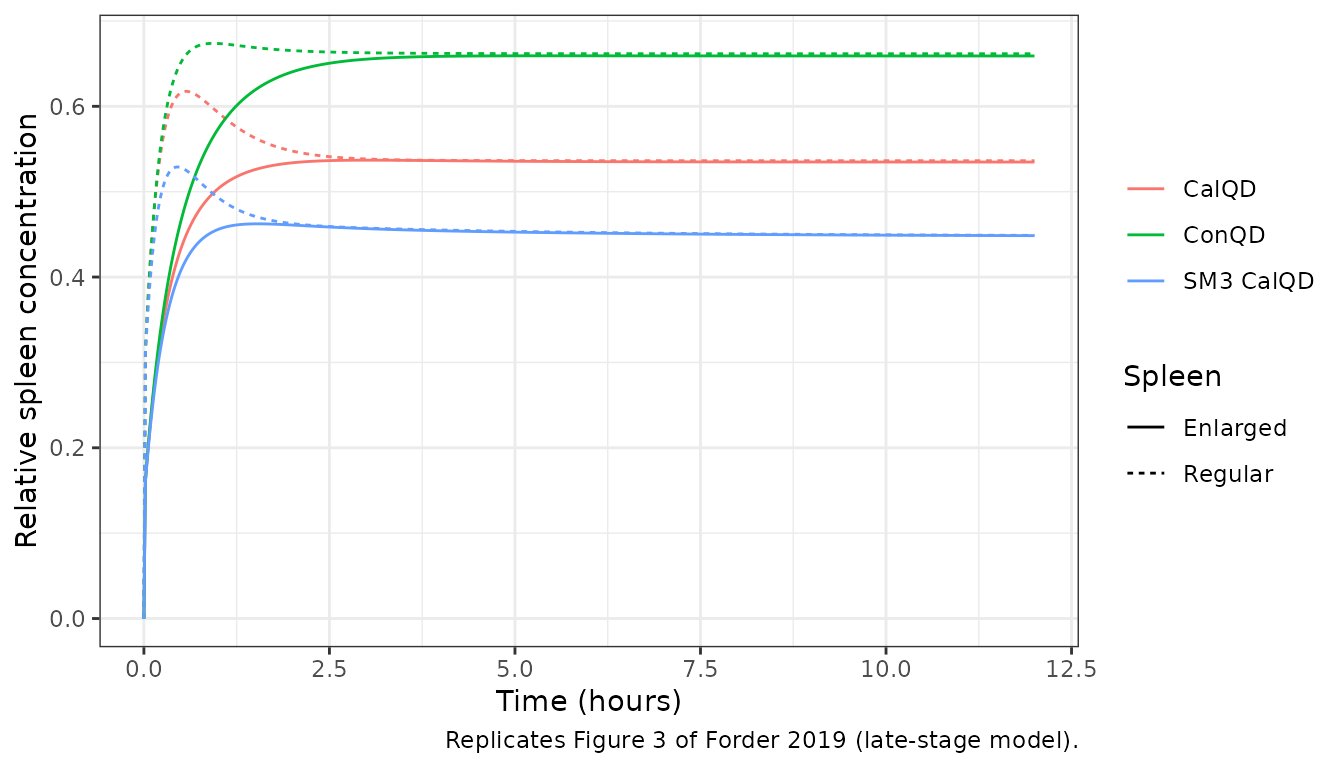

As the paper notes, the early spleen peak disappears when the spleen volume is doubled and its blood flow is kept the same.

Replicating Figure S3 (SM3 CalQD over 4 days)

figS3 <- bind_rows(lapply(names(stages), function(st) {
  norm(sm3(st)) |>
    filter(compartment != "plasma", compartment != "other") |>
    mutate(stage = factor(st, levels = names(stages)))
}))
ggplot(figS3, aes(time, rel, colour = compartment)) +
  geom_line() +
  facet_wrap(~stage) +
  labs(
    x = "Time (hours)", y = "Relative concentration (C / C_plasma,0)",
    colour = NULL, caption = "Replicates Figure S3 of Forder 2019."
  ) +
  theme_bw()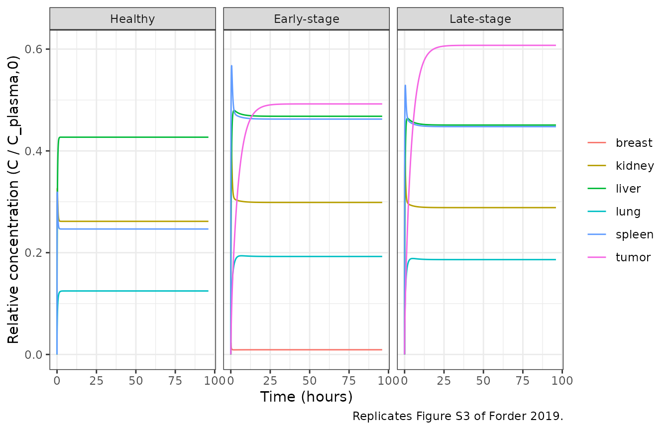

PKNCA: tissue exposure over 0-96 h

The paper reports no NCA, so there is no published table to compare against. PKNCA is used to summarise each tissue’s Cmax, Tmax and AUC over 0-96 h for the three SM3 CalQD models (the paper’s main case). The grouping includes the disease stage.

nca_in <- bind_rows(lapply(names(stages), function(st) {
  sm3(st) |>
    select(id, time, kidney, liver, spleen, lung, any_of("tumor")) |>
    pivot_longer(-c(id, time), names_to = "tissue", values_to = "conc") |>
    mutate(stage = st)
})) |>
  filter(!is.na(conc))

dose_df <- expand.grid(
  id = 1L, stage = names(stages),
  tissue = c("kidney", "liver", "spleen", "lung", "tumor"),
  stringsAsFactors = FALSE
) |>
  semi_join(distinct(nca_in, stage, tissue), by = c("stage", "tissue")) |>
  mutate(time = 0, amt = dose_pmol)

conc_obj <- PKNCA::PKNCAconc(nca_in, conc ~ time | stage + tissue / id)
dose_obj <- PKNCA::PKNCAdose(dose_df, amt ~ time | stage + tissue + id, route = "intravascular")
intervals <- data.frame(start = 0, end = 96, cmax = TRUE, tmax = TRUE, auclast = TRUE)
nca_res <- PKNCA::pk.nca(PKNCA::PKNCAdata(conc_obj, dose_obj, intervals = intervals))
nca_tab <- as.data.frame(nca_res) |>
  select(stage, tissue, PPTESTCD, PPORRES) |>
  pivot_wider(names_from = PPTESTCD, values_from = PPORRES)
knitr::kable(
  nca_tab |>
    rename(
      Stage = stage, Tissue = tissue, "Cmax (nM)" = cmax,
      "Tmax (h)" = tmax, "AUC0-96 (nM*h)" = auclast
    ),
  digits = 3
)

Stage	Tissue	AUC0-96 (nM*h)	Cmax (nM)	Tmax (h)
Early-stage	kidney	1152.205	16.764	0.30
Early-stage	liver	1795.491	19.180	2.08
Early-stage	lung	734.790	7.757	6.80
Early-stage	spleen	1781.687	22.700	0.50
Early-stage	tumor	1808.777	19.692	59.75
Healthy	kidney	1005.733	13.061	0.18
Healthy	liver	1636.191	17.079	2.58
Healthy	lung	477.700	4.991	7.98
Healthy	spleen	948.071	12.763	0.14
Late-stage	kidney	1112.177	15.302	0.26
Late-stage	liver	1730.070	18.565	1.86
Late-stage	lung	712.271	7.543	5.14
Late-stage	spleen	1723.878	21.158	0.46
Late-stage	tumor	2238.385	24.298	56.50

stopifnot(nrow(nca_tab) == 14, !anyNA(nca_tab$cmax))

Assumptions and deviations (Errata)

• Deposited code is used where it differs from the printed equations. The supplementary MATLAB code reproduces all nine Table 3 fits (and all six Table S2 fits) against Table 2. Where the code differs from the printed equations, the printed forms do not reproduce the fits, so the code is used:
  • Late-stage plasma (Eq. 14). The code returns q_liver * liver / kp_liver + q_spleen * spleen / kp_spleen to plasma. The printed Eq. 14 returns (q_liver + q_spleen) * liver / kp_liver. Spleen outflow is therefore counted twice in the code, since the liver equation receives it as well. This creates 1.0-3.6% spurious mass (depending on the QD) over the first hours (the net creation q_spleen * (spleen/kp_spleen - liver/kp_liver) goes to zero at equilibrium). The printed equation conserves mass but under-predicts Table 2 by about 3.5% for SM3 CalQD with the Table 3 partition coefficients (see “Mass balance”).
  • Early-stage breast and tumor (Eq. 19-20). In the code the tumor is fed at the breast venous concentration breast / kp_breast, and the breast loses q_tumor at that same concentration. The printed equations drop / kp_breast from both terms. Both forms conserve mass, but only the code form reproduces the early-stage ConQD and CalQD fits.
• Early-stage SM3 CalQD partition coefficients. The Table 3 column equals the Table S2 enlarged-spleen column, and these values reproduce Table 2 only with a doubled spleen volume. The model ships them as printed, with the regular spleen volume, and they over-predict Table 2 by about 3%. Nothing was refitted. For the enlarged-spleen case, set v_spleen = 0.154.
• Other-tissue flow. The code uses q_other = 700.3091 mL/h for the healthy and late-stage models and 677.5191 mL/h for the early-stage model, where the 22.79 mL/h breast flow is subtracted. Table 1 prints only the early-stage 677.5, but its 944.3 mL/h plasma total equals the sum of flows with 700.3. The text says the breast volume is subtracted from other, but the code (and Table 1’s 55.76 mL) keeps v_other unchanged in every model, and the code is what is followed here.
• Liver elimination units. Eq. 3 quotes kelim in 1/h, but Eq. 12 and the code multiply it by the liver concentration inside the 1/V_liver bracket. It therefore behaves as a clearance of 1e-6 mL/h. Either way it is negligible over the simulated horizon.
• Concentration scale. The fit targets are fluorescence pixel intensities (Table 2). The code labels them nM and starts plasma at 40 nM, and that scale is kept here (dose 43.12 pmol into 1.078 mL). Because the model is linear, the dose only scales the output. The relative concentrations in Figures 2, 3 and S3 do not depend on it.
• Stray lines in the deposited code. Both tumor-model scripts carry an active vs = 2*0.077 (enlarged spleen) line, left over from the Table S2 runs. The regular-spleen Table 3 fits reproduce only with vs = 0.077, so that value is used.
• Sensitivity analysis not shipped as models. The enlarged-spleen (Table S2) fits are reproduced above by ini() override, not packaged separately.
• No variability. The fits were relative least squares against mean intensities, with no uncertainty or variance components. The models are for typical-value simulation only.