Indian F(ab')2 snake antivenom (Isbister 2015)
Source:vignettes/articles/Isbister_2015_snake_antivenom.Rmd
Isbister_2015_snake_antivenom.RmdModel and source
- Citation: Isbister GK, Maduwage K, Saiao A, Buckley NA, Jayamanne SF, Seyed S, Mohamed F, Chathuranga U, Mendes A, Abeysinghe C, Karunathilake H, Gawarammana I, Lalloo DG, de Silva HJ. Population Pharmacokinetics of an Indian F(ab’)2 Snake Antivenom in Patients with Russell’s Viper (Daboia russelii) Bites. PLoS Negl Trop Dis. 2015;9(7):e0003873. doi:10.1371/journal.pntd.0003873.
- Description: Two-compartment population PK model for Indian polyvalent F(ab’)2 snake antivenom (VINS Bioproducts Ltd) in adults with Russell’s viper (Daboia russelii) envenoming (Isbister 2015): zero-order intravenous input, linear elimination from the central compartment, and a power effect of body weight on central volume. Relative bioavailability is fixed to 1 with between-subject variability estimated; that random effect absorbs the per-patient uncertainty in the delivered antivenom dose caused by variable losses during reconstitution of the freeze-dried vials. Fit in MONOLIX 4.2 (SAEM, M3 handling of below-limit-of-quantification data) to 411 quantifiable antivenom concentrations from 75 patients. The authors selected a combined (additive plus proportional) residual-error model but publish no residual-error magnitudes, so both are encoded as zero.
- Article: https://doi.org/10.1371/journal.pntd.0003873
Isbister and colleagues measured serial serum antivenom concentrations in patients treated for Russell’s viper envenoming in Sri Lanka and fit a population PK model in MONOLIX 4.2. The final model is two-compartment with zero-order intravenous input and linear elimination, a power effect of body weight on the central volume, and between-subject variability on a relative bioavailability term that was itself fixed to 1 so that the random effect carries the per-patient uncertainty in the delivered dose.
Population
The analysis used 75 patients (Table 1) admitted to Base Hospital Polonnaruwa between October 2010 and March 2012 with a suspected snake bite and coagulopathy. Median age was 38 years (16 to 64), median weight 57 kg (40 to 70), and 64 of 75 (85%) were male. Seventy-one had Russell’s viper envenoming (52 with venom detectable before antivenom) and four had hump-nosed viper (Hypnale spp.) envenoming. All received Indian polyvalent antivenom (VINS Bioproducts Ltd) intravenously; the median dose was 18 vials (range 8 to 40) and 21 patients (28%) received a repeat dose. Each 10-vial dose is reconstituted in 100 mL and infused in a total of 500 mL of normal saline over 1 hour.
Of 510 samples drawn, 411 had quantifiable antivenom (limit of quantification 40 ug/mL); the 54 single-dose patients contributed a median of 5 samples each and the 21 multiple-dose patients a median of 7.
The same information is available programmatically via
readModelDb("Isbister_2015_snake_antivenom")()$population.
Source trace
Every ini() entry in
inst/modeldb/specificDrugs/Isbister_2015_snake_antivenom.R
carries an in-file comment pointing at its origin. They are collected
here for review. All structural and variability values come from the
Model 3 (Final) column of Table 2.
| Equation / parameter | Value | Source location |
|---|---|---|
lcl (CL) |
0.0779 L/h | Table 2, Model 3 (Final), row CL (Lh-1), rse 34% |
lvc (V) |
2.16 L | Table 2, Model 3 (Final), row V (L), rse 10% |
lq (Q) |
0.178 L/h | Table 2, Model 3 (Final), row Q (Lh-1), rse 31% |
lvp (Vp) |
8.33 L | Table 2, Model 3 (Final), row Vp (L), rse 52% |
e_wt_vc (f_wt) |
0.132 | Table 2, Model 3 (Final), row fwt, rse 84% |
lfdepot (F) |
1 (fixed) | Table 2, Model 3 (Final), row F; Methods: “F was fixed
to 1 and the BSV was estimated for each patient” |
etalcl |
0.715 (SD) | Table 2, Between subject variance block, row Cl, rse
46% |
etalvc |
0.188 (SD) | Table 2, Between subject variance block, row V, rse
126% |
etalq |
0.533 (SD) | Table 2, Between subject variance block, row Q, rse
57% |
etalvp |
0.836 (SD) | Table 2, Between subject variance block, row Vp, rse
125% |
etalfdepot |
0.197 (SD) | Table 2, Between subject variance block, row F, rse
42% |
propSd, addSd
|
0 (not published) | Results: “a combined error model best described the data”; no magnitude appears in Table 2 or in supporting files S1 to S5 |
V = theta_V * (wt/wt_av)^f_wt |
n/a | Methods, “Pharmacokinetic analysis”, unnumbered equation |
| Two-compartment disposition, zero-order input, linear elimination | n/a | Methods, “Pharmacokinetic analysis”; Results, “Pharmacokinetic analysis” |
Reference weight wt_av = 57 kg
|
57 kg | Table 1 median weight (the paper centres on the “average weight” but never prints it; see Assumptions) |
Scale of the between-subject variability terms
Table 2’s variability block is headed Between subject
variance but the values are MONOLIX 4.2
omega_<parameter> outputs, which are the
standard deviations of the log-normal random effects.
The model therefore encodes each as omega^2. Three
independent checks agree on that reading:
- MONOLIX 4.2 reports
omega_Xas an SD. - The SD reading reproduces the paper’s own reported half-life distribution (checked numerically below); the variance reading over-disperses both half-lives by roughly a further 50%.
-
omega_F = 0.197as an SD is a 20% CV in the delivered dose, matching the authors’ stated mechanism (“variable losses occurring during reconstitution of the individual freeze dried vials”). As a variance it would be a 47% CV, far larger than reconstitution losses can plausibly be.
Dose units
The paper never reports the antivenom mass per vial: doses are given in vials throughout, and the assay’s standard curve was built from “serial dilutions of antivenom”, so the reported ug/mL are in units of the antivenom calibrator. To simulate, a mass per vial is needed. It can be recovered from Figure 2, which plots concentration versus time for a 10-vial dose given over 20 min, 1 h and 2 h: solving the published two-compartment model for the dose that reproduces those peaks fixes the scale.
# Typical-value parameters, Table 2 Model 3 (Final).
CL <- 0.0779; V <- 2.16; Q <- 0.178; VP <- 8.33
k10 <- CL / V; k12 <- Q / V; k21 <- Q / VP
aa <- k10 + k12 + k21; bb <- k10 * k21
dd <- sqrt(aa^2 - 4 * bb)
lam1 <- (aa + dd) / 2   # distribution (fast) eigenvalue, 1/h
lam2 <- (aa - dd) / 2   # elimination (slow) eigenvalue, 1/h

# Central concentration at the end of a zero-order infusion of rate R, length Tinf.
conc_end_inf <- function(Tinf, R) {
  A <- R / V * (k21 - lam1) / (lam1 * (lam2 - lam1))
  B <- R / V * (k21 - lam2) / (lam2 * (lam1 - lam2))
  A * (1 - exp(-lam1 * Tinf)) + B * (1 - exp(-lam2 * Tinf))
}

# Median peaks read off Figure 2 for the 10-vial dose (ug/mL): panels B, C and
# D give the median curve for each infusion duration, and panel A overlays all
# three. Resolution of reading a peak off the printed axis is about +/-3%.
fig2_peaks <- c(`20 min` = 9500, `1 h` = 9000, `2 h` = 7800)
tinf       <- c(`20 min` = 20 / 60, `1 h` = 1, `2 h` = 2)
dose_10vials <- fig2_peaks / vapply(tinf, function(t) conc_end_inf(t, 1 / t), numeric(1))

backsolve_tbl <- tibble::tibble(
  Infusion  = names(tinf),
  `Fig 2 peak (ug/mL)` = as.numeric(fig2_peaks),
  `Implied 10-vial dose (mg)` = round(as.numeric(dose_10vials)),
  `Implied mg per vial` = round(as.numeric(dose_10vials) / 10)
)
knitr::kable(backsolve_tbl, caption = "Back-solving the antivenom mass per vial from Figure 2.")| Infusion | Fig 2 peak (ug/mL) | Implied 10-vial dose (mg) | Implied mg per vial |
|---|---|---|---|
| 20 min | 9500 | 20927 | 2093 |
| 1 h | 9000 | 20608 | 2061 |
| 2 h | 7800 | 18901 | 1890 |
# The three panels imply 2093, 2061 and 1890 mg per vial - agreement to within
# about 6%, despite the model predicting per-unit-dose peaks that differ by 10%
# across the three durations. Round to a single working value.
MG_PER_VIAL <- 2000
DOSE_10VIALS <- 10 * MG_PER_VIAL

stopifnot(
  # The three independently-read panels must agree that the vial mass is of
  # order 2 g; a mis-transcribed V or CL would scatter them or move them all
  # by a factor, not leave them clustered around the same value. This is a
  # genuine consistency check on the structural parameters, not just on the
  # figure reading: the three infusion durations exercise different parts of
  # the biexponential input response.
  all(abs(dose_10vials / 10 / MG_PER_VIAL - 1) < 0.10)
)
A vial is therefore about 2 g of assay-calibrator-equivalent antivenom, and the 10-vial dose used in Figures 2 and 3 is about 20 g. This is a figure-derived convenience, not a paper-reported value - see Assumptions and deviations. It is also a consistency check on the model itself: 2 g/vial applied to the median 18-vial clinical dose gives an expected peak near 16,000 ug/mL, against a maximum observed concentration of 13,673 ug/mL (Table 1).
Virtual cohort
Original data are not redistributed here (the authors deposited them at http://hdl.handle.net/1959.13/1063469). The cohorts below sample body weight to match the published distribution: median 57 kg, range 40 to 70 kg (Table 1).
# set.seed() seeds R's RNG, not rxode2's. rxode2's streams are partitioned per
# solver thread, so this cohort is reproducible on this machine and different
# on a machine with a different thread count. Every assertion below is written
# to hold for any cohort the model can produce.
set.seed(20150702)
rxode2::rxSetSeed(20150702)

N_PER_ARM <- 150

sample_weight <- function(n) {
  # Log-normal centred on the published median, truncated to the published
  # 40-70 kg range. The paper reports no SD, so 15% CV is assumed.
  pmin(pmax(stats::rlnorm(n, meanlog = log(57), sdlog = 0.15), 40), 70)
}

# One arm = N_PER_ARM subjects given `n_vials` vials over `tinf` hours,
# optionally repeated after `repeat_h` hours.
make_arm <- function(label, tinf, n_vials = 10, repeat_h = NA_real_,
                     obs_times = seq(0, 24, by = 0.25), id_offset = 0L) {
  subj <- tibble::tibble(
    id  = id_offset + seq_len(N_PER_ARM),
    WT  = sample_weight(N_PER_ARM),
    arm = label
  )
  dose_times <- if (is.na(repeat_h)) 0 else c(0, repeat_h)
  amt <- n_vials * MG_PER_VIAL
  doses <- tidyr::crossing(subj, time = dose_times) |>
    dplyr::mutate(amt = amt, evid = 1L, rate = amt / tinf, cmt = "central")
  obs <- tidyr::crossing(subj, time = obs_times) |>
    dplyr::mutate(amt = NA_real_, evid = 0L, rate = NA_real_, cmt = "central")
  dplyr::bind_rows(doses, obs) |> dplyr::arrange(id, time, dplyr::desc(evid))
}

# Figure 2: one 10-vial dose at three infusion durations.
ev_fig2 <- dplyr::bind_rows(
  make_arm("20 min", tinf = 20 / 60, id_offset =   0L),
  make_arm("1 h",    tinf = 1,       id_offset = 200L),
  make_arm("2 h",    tinf = 2,       id_offset = 400L)
)

# Figure 3: two 10-vial doses each over 1 h, 6 h or 12 h apart, against the
# single-dose reference.
ev_fig3 <- dplyr::bind_rows(
  make_arm("1 dose",          tinf = 1,                    id_offset =  600L),
  make_arm("2 doses, 6 h",    tinf = 1, repeat_h =  6,     id_offset =  800L),
  make_arm("2 doses, 12 h",   tinf = 1, repeat_h = 12,     id_offset = 1000L)
)

# NCA cohort: single 10-vial 1 h infusion followed far enough out to
# characterise the terminal phase (the typical terminal half-life is about
# 120 h, so 1000 h is roughly eight half-lives).
nca_times <- sort(unique(c(
  seq(0, 4, by = 0.1), seq(4, 24, by = 0.5), seq(24, 240, by = 6),
  seq(240, 1000, by = 24)
)))
ev_nca <- make_arm("10 vials, 1 h", tinf = 1, obs_times = nca_times,
                   id_offset = 2000L)

stopifnot(
  !anyDuplicated(dplyr::distinct(ev_fig2, id, time, evid)),
  length(intersect(ev_fig2$id, ev_fig3$id)) == 0L,
  length(intersect(ev_fig2$id, ev_nca$id)) == 0L
)
Simulation
mod <- readModelDb("Isbister_2015_snake_antivenom")

sim_fig2 <- rxode2::rxSolve(mod, events = as.data.frame(ev_fig2), keep = c("arm", "WT")) |>
  as.data.frame()
#> ℹ parameter labels from comments will be replaced by 'label()'
sim_fig3 <- rxode2::rxSolve(mod, events = as.data.frame(ev_fig3), keep = c("arm", "WT")) |>
  as.data.frame()
sim_nca  <- rxode2::rxSolve(mod, events = as.data.frame(ev_nca),  keep = c("arm", "WT")) |>
  as.data.frame()

# Typical-value (no between-subject variability) solve of the same Figure 2
# design, for the deterministic checks below.
mod_typ <- rxode2::zeroRe(mod)
#> ℹ parameter labels from comments will be replaced by 'label()'
sim_fig2_typ <- rxode2::rxSolve(
  mod_typ,
  events = as.data.frame(dplyr::filter(ev_fig2, id %in% c(1L, 201L, 401L))),
  keep = c("arm", "WT")
) |> as.data.frame()
#> ℹ omega/sigma items treated as zero: 'etalcl', 'etalvc', 'etalq', 'etalvp', 'etalfdepot'
#> Warning: multi-subject simulation without without 'omega'

stopifnot(nrow(sim_fig2) > 0, !anyNA(sim_fig2$Cc), all(sim_fig2$Cc >= 0))
Replicate published figures
# Replicates Figure 2 of Isbister 2015: median and 10th/90th percentile
# concentrations for a single 10-vial dose over 20 min, 1 h and 2 h.
fig2_bands <- sim_fig2 |>
  dplyr::group_by(arm, time) |>
  dplyr::summarise(
    Q10 = quantile(Cc, 0.10), Q50 = median(Cc), Q90 = quantile(Cc, 0.90),
    .groups = "drop"
  )

ggplot(fig2_bands, aes(time, Q50)) +
  geom_ribbon(aes(ymin = Q10, ymax = Q90), alpha = 0.2) +
  geom_line(linewidth = 0.7) +
  facet_wrap(~arm) +
  labs(
    x = "Time (hours)", y = "Antivenom concentration (ug/mL)",
    title = "Figure 2 - one 10-vial dose at three infusion durations",
    caption = "Median with 10th-90th percentiles. Replicates Figure 2 of Isbister 2015."
  ) +
  theme_bw()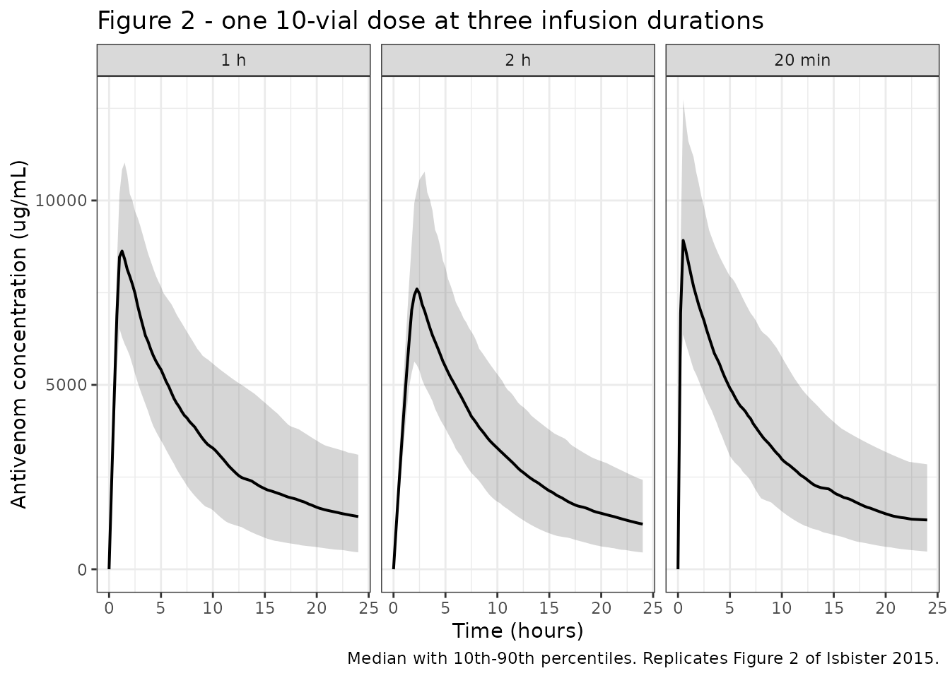
Replicates Figure 2 of Isbister 2015.
# Figure 2A compares the three median curves directly: a slower infusion gives
# a slightly lower and later peak. Checked on the TYPICAL-VALUE solve, where
# the comparison is deterministic rather than a race between three noisy
# cohort medians.
peaks_typ <- sim_fig2_typ |>
  dplyr::group_by(arm) |>
  dplyr::summarise(Cmax = max(Cc), Tmax = time[which.max(Cc)], .groups = "drop") |>
  dplyr::arrange(match(arm, c("20 min", "1 h", "2 h")))

knitr::kable(
  peaks_typ |>
    dplyr::rename("Infusion" = arm, "Typical Cmax (ug/mL)" = Cmax, "Typical Tmax (h)" = Tmax),
  digits = c(0, 0, 2),
  caption = "Typical-value peak for a 10-vial dose (Figure 2A of Isbister 2015)."
)| Infusion | Typical Cmax (ug/mL) | Typical Tmax (h) |
|---|---|---|
| 20 min | 8977 | 0.5 |
| 1 h | 8758 | 1.0 |
| 2 h | 8256 | 2.0 |
stopifnot(
  # The paper's claim: "a slightly lower and later peak with slower infusions".
  # Deterministic on the typical-value solve.
  all(diff(peaks_typ$Cmax) < 0),
  all(diff(peaks_typ$Tmax) > 0),
  # "Slightly": the 2 h peak stays within 20% of the 20 min peak. The paper's
  # own Figure 2A shows roughly a 20% spread across the three curves.
  peaks_typ$Cmax[3] / peaks_typ$Cmax[1] > 0.80
)
# Replicates Figure 3 of Isbister 2015: two 10-vial doses 6 h or 12 h apart,
# compared with a single dose.
fig3_bands <- sim_fig3 |>
  dplyr::group_by(arm, time) |>
  dplyr::summarise(
    Q10 = quantile(Cc, 0.10), Q50 = median(Cc), Q90 = quantile(Cc, 0.90),
    .groups = "drop"
  )

ggplot(fig3_bands, aes(time, Q50, colour = arm, fill = arm)) +
  geom_ribbon(aes(ymin = Q10, ymax = Q90), alpha = 0.15, colour = NA) +
  geom_line(linewidth = 0.7) +
  labs(
    x = "Time (hours)", y = "Antivenom concentration (ug/mL)",
    colour = NULL, fill = NULL,
    title = "Figure 3 - repeat dosing at 6 h and 12 h",
    caption = "Median with 10th-90th percentiles. Replicates Figure 3 of Isbister 2015."
  ) +
  theme_bw() +
  theme(legend.position = "bottom")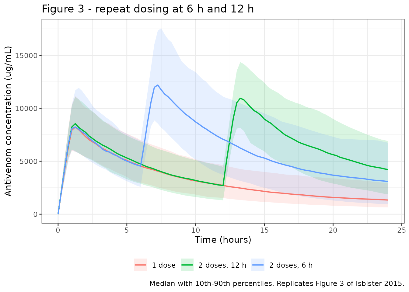
Replicates Figure 3 of Isbister 2015.
# Paper: "antivenom concentrations decrease rapidly after each dose and there
# are low but persistent levels of antivenom after one dose and both two dose
# regimens."
c24 <- sim_fig3 |>
  dplyr::filter(abs(time - 24) < 1e-8) |>
  dplyr::group_by(arm) |>
  dplyr::summarise(c24 = median(Cc), .groups = "drop")

cmax_by_arm <- sim_fig3 |>
  dplyr::group_by(arm, id) |>
  dplyr::summarise(Cmax = max(Cc), .groups = "drop") |>
  dplyr::group_by(arm) |>
  dplyr::summarise(cmax = median(Cmax), .groups = "drop")

# Join BY NAME. Two independent group_by(arm) |> summarise() calls happen to
# emit rows in the same (alphabetical) order here, but dividing one column by
# the other positionally would silently compare the wrong arms the moment an
# arm is renamed or added.
fig3_tbl <- dplyr::left_join(cmax_by_arm, c24, by = "arm") |>
  dplyr::mutate(ratio = c24 / cmax)

knitr::kable(
  fig3_tbl |>
    dplyr::rename(
      "Regimen" = arm,
      "Median Cmax (ug/mL)" = cmax,
      "Median Cc at 24 h (ug/mL)" = c24,
      "24 h / Cmax" = ratio
    ),
  digits = c(0, 0, 0, 3),
  caption = "Repeat-dose exposure summary (Figure 3 of Isbister 2015)."
)| Regimen | Median Cmax (ug/mL) | Median Cc at 24 h (ug/mL) | 24 h / Cmax |
|---|---|---|---|
| 1 dose | 8444 | 1338 | 0.158 |
| 2 doses, 12 h | 11237 | 4214 | 0.375 |
| 2 doses, 6 h | 12395 | 3079 | 0.248 |
stopifnot(
  nrow(fig3_tbl) == 3L,
  # "Low but persistent levels" at 24 h: above the 40 ug/mL assay limit of
  # quantification in every arm.
  all(fig3_tbl$c24 > 40),
  # "Concentrations decrease rapidly after each dose": by 24 h every arm sits
  # well under half its own peak. The bound has to accommodate the 12 h repeat
  # arm, whose second dose is only 12 h old at the readout and has therefore
  # decayed through barely two distribution half-lives (realised ratio ~0.37).
  all(fig3_tbl$ratio < 0.5),
  # The single-dose arm is the clean test of the decline - one 1 h infusion
  # followed by 23 h of decay through a 5 h distribution phase into the slow
  # phase - so it is gated tightly. Nothing here depends on repeat-dose timing.
  fig3_tbl$ratio[fig3_tbl$arm == "1 dose"] < 0.25,
  # Ordering: the more recently the last dose was given, the higher the 24 h
  # level. This is a structural gate on the repeat-dose event table - a dose
  # placed at the wrong time, or silently dropped, breaks the ordering.
  fig3_tbl$c24[fig3_tbl$arm == "2 doses, 12 h"] >
    fig3_tbl$c24[fig3_tbl$arm == "2 doses, 6 h"],
  fig3_tbl$c24[fig3_tbl$arm == "2 doses, 6 h"] >
    fig3_tbl$c24[fig3_tbl$arm == "1 dose"]
)
Half-life checks
The paper’s headline dispositional result is a median distribution half-life of 4.6 h (10th-90th percentiles 2.6 to 7.1) and a median elimination half-life of 140 h (95 to 223). Both are medians of the individual (empirical Bayes) estimates, so their spread is shrunk relative to the population the model describes; the medians, however, are directly comparable.
# Closed form for the typical patient (WT = 57 kg, so the weight term is 1).
typ_hl <- c(distribution = log(2) / lam1, elimination = log(2) / lam2)

# Per-subject half-lives across the simulated cohort, from each subject's own
# parameters (rxSolve returns cl / vc / q / vp per subject).
subj_par <- sim_nca |>
  dplyr::distinct(id, cl, vc, q, vp) |>
  dplyr::mutate(
    a  = cl / vc + q / vc + q / vp,
    b  = (cl / vc) * (q / vp),
    d  = sqrt(a^2 - 4 * b),
    l1 = (a + d) / 2,
    l2 = (a - d) / 2,
    t_half_dist = log(2) / l1,
    t_half_elim = log(2) / l2
  )

hl_tbl <- tibble::tibble(
  Quantity = c("Distribution half-life (h)", "Elimination half-life (h)"),
  `Typical value` = round(as.numeric(typ_hl), 1),
  `Cohort median` = round(c(median(subj_par$t_half_dist), median(subj_par$t_half_elim)), 1),
  `Cohort 10th-90th` = c(
    paste(round(quantile(subj_par$t_half_dist, c(0.1, 0.9)), 1), collapse = " to "),
    paste(round(quantile(subj_par$t_half_elim, c(0.1, 0.9)), 0), collapse = " to ")
  ),
  `Published median` = c(4.6, 140),
  `Published 10th-90th` = c("2.6 to 7.1", "95 to 223")
)
knitr::kable(hl_tbl, caption = "Simulated versus published half-lives (Isbister 2015, Results).")| Quantity | Typical value | Cohort median | Cohort 10th-90th | Published median | Published 10th-90th |
|---|---|---|---|---|---|
| Distribution half-life (h) | 5.2 | 4.6 | 2.5 to 7.9 | 4.6 | 2.6 to 7.1 |
| Elimination half-life (h) | 120.6 | 128.1 | 39 to 456 | 140.0 | 95 to 223 |
stopifnot(
  # Structural gate on the CENTRE. A mis-transcribed CL, Q, V or Vp moves these
  # medians by tens of percent; the realised values are near 4.6 h and 133 h,
  # so 35% leaves headroom for cohort noise while still going red on a
  # transcription error.
  abs(median(subj_par$t_half_dist) / 4.6 - 1) < 0.35,
  abs(median(subj_par$t_half_elim) / 140 - 1) < 0.35,
  # The typical-value closed form must bracket the same region.
  typ_hl[["distribution"]] > 3 && typ_hl[["distribution"]] < 8,
  typ_hl[["elimination"]] > 90 && typ_hl[["elimination"]] < 200
)
The cohort’s 10th-90th percentile range is wider than the published one, as expected: the published range summarises shrunk individual estimates from 411 observations across 75 patients, whereas the simulation draws from the full estimated between-subject distribution. Reading the Table 2 variability terms as variances rather than SDs widens the simulated range by roughly a further 50% while leaving the medians in place, which is the second of the three checks cited in the Source trace section.
PKNCA validation
# IMPORTANT: filter on !is.na(Cc) only - a `time > 0` or `Cc > 0` filter would
# drop the time-zero row PKNCA needs to anchor AUC0-*.
conc_df <- sim_nca |>
  dplyr::filter(!is.na(Cc)) |>
  dplyr::select(id, time, Cc, arm)

conc_df <- dplyr::bind_rows(
  conc_df,
  conc_df |> dplyr::distinct(id, arm) |> dplyr::mutate(time = 0, Cc = 0)
) |>
  dplyr::distinct(id, arm, time, .keep_all = TRUE) |>
  dplyr::arrange(id, time)

dose_df <- ev_nca |>
  dplyr::filter(evid == 1L) |>
  dplyr::select(id, time, amt, arm)

conc_obj <- PKNCA::PKNCAconc(conc_df, Cc ~ time | arm + id,
                             concu = "ug/mL", timeu = "h")
dose_obj <- PKNCA::PKNCAdose(dose_df, amt ~ time | arm + id, doseu = "mg")

intervals <- data.frame(
  start = 0, end = Inf,
  cmax = TRUE, tmax = TRUE, aucinf.obs = TRUE, half.life = TRUE,
  clast.obs = TRUE, lambda.z = TRUE
)

nca_res <- PKNCA::pk.nca(PKNCA::PKNCAdata(conc_obj, dose_obj, intervals = intervals))
nca_tbl <- as.data.frame(nca_res$result)
stopifnot(nrow(nca_tbl) > 0)
Mass balance
With relative bioavailability fixed to 1, the entire administered
dose must clear through CL, so AUC(0-inf) * CL = Dose
exactly for each subject. This is a deterministic identity, checked here
as a closed-form gate on the simulation and the NCA together.
auc_by_id <- nca_tbl |>
  dplyr::filter(PPTESTCD == "aucinf.obs") |>
  dplyr::select(id, aucinf = PPORRES)

mb <- subj_par |>
  dplyr::select(id, cl) |>
  dplyr::left_join(auc_by_id, by = "id") |>
  dplyr::left_join(
    sim_nca |> dplyr::distinct(id, fdepot), by = "id"
  ) |>
  dplyr::mutate(
    delivered = DOSE_10VIALS * fdepot,
    recovered = aucinf * cl,
    pct_diff  = 100 * (recovered - delivered) / delivered
  )

stopifnot(
  nrow(mb) == N_PER_ARM,
  !anyNA(mb$pct_diff),
  # Pure numerical error: both sides use the SAME drawn parameters, so this is
  # trapezoidal + terminal-extrapolation error only and a tight all() bound is
  # correct here.
  max(abs(mb$pct_diff)) < 3
)

knitr::kable(
  tibble::tibble(
    Quantity = "AUC(0-inf) x CL vs delivered dose",
    `Median % difference` = round(median(mb$pct_diff), 3),
    `Max abs % difference` = round(max(abs(mb$pct_diff)), 3)
  ),
  caption = "Mass balance: every subject's AUC(0-inf) x CL must equal their delivered dose."
)| Quantity | Median % difference | Max abs % difference |
|---|---|---|
| AUC(0-inf) x CL vs delivered dose | 0.014 | 0.239 |
Comparison against published NCA
Isbister 2015 reports no NCA table, but it does report the two
disposition half-lives, which PKNCA’s half.life (the
terminal, elimination half-life) can be compared against directly.
published <- tibble::tibble(
  arm = "10 vials, 1 h",
  half.life = 140      # Results: median elimination half-life 140 h
)

cmp <- nlmixr2lib::ncaComparisonTable(
  simulated     = nca_res,
  reference     = published,
  by            = "arm",
  params        = "half.life",
  units         = c(half.life = "h"),
  tolerance_pct = 20
)

knitr::kable(
  cmp,
  caption = "Simulated (cohort median) versus published NCA. * differs from reference by >20%."
)| NCA parameter | arm | Reference | Simulated | % diff |
|---|---|---|---|---|
| t½ (h) | 10 vials, 1 h | 140 | 128 | -8.8% |
nca_summary <- nca_tbl |>
  dplyr::filter(PPTESTCD %in% c("cmax", "tmax", "aucinf.obs", "half.life")) |>
  dplyr::group_by(PPTESTCD) |>
  dplyr::summarise(
    Median = median(PPORRES, na.rm = TRUE),
    `10th` = quantile(PPORRES, 0.10, na.rm = TRUE),
    `90th` = quantile(PPORRES, 0.90, na.rm = TRUE),
    .groups = "drop"
  ) |>
  dplyr::mutate(PPTESTCD = dplyr::recode(
    PPTESTCD,
    cmax = "Cmax (ug/mL)", tmax = "Tmax (h)",
    aucinf.obs = "AUC0-inf (ug*h/mL)", half.life = "t1/2 (h)"
  ))

knitr::kable(
  nca_summary |> dplyr::rename("NCA parameter" = PPTESTCD),
  digits = 1,
  caption = "Simulated NCA for a single 10-vial (about 20 g) 1 h infusion, n = 150."
)| NCA parameter | Median | 10th | 90th |
|---|---|---|---|
| AUC0-inf (ug*h/mL) | 245777.5 | 96247.0 | 647605.0 |
| Cmax (ug/mL) | 8462.1 | 5956.8 | 11644.1 |
| t1/2 (h) | 127.7 | 39.0 | 455.1 |
| Tmax (h) | 1.0 | 0.8 | 1.3 |
stopifnot(
  # Cmax for a 20 g dose into a 2.16 L central volume lands near 9000 ug/mL;
  # the maximum concentration ever observed in the study was 13,673 ug/mL for
  # doses up to 40 vials (Table 1), so a cohort median well outside
  # 5,000-15,000 would mean the dose scale or the volume is wrong.
  dplyr::between(nca_summary$Median[nca_summary$PPTESTCD == "Cmax (ug/mL)"], 5000, 15000),
  # The PKNCA terminal half-life and the eigenvalue-derived one must agree;
  # both describe the same terminal slope.
  abs(nca_summary$Median[nca_summary$PPTESTCD == "t1/2 (h)"] /
        median(subj_par$t_half_elim) - 1) < 0.15
)
Assumptions and deviations
-
Between-subject variability scale. Table 2’s block
is headed Between subject variance but the values are MONOLIX
omega_Xoutputs, i.e. standard deviations. The model encodesomega^2. See the Source trace section for the three checks that settle this; the reading changes the simulated half-life spread by about 50% but not the medians. -
Reference weight. The Methods say the weight
covariate was “centred to the average weight” but never print the
average. Table 1 reports only the median weight, 57 kg,
which is what the model uses for
wt_av. The exponent is small (0.132) and the cohort weight range narrow (40 to 70 kg), so the choice moves the central volume by at most about 4% across the range; a different centring constant would rescaleVby(57/wt_av)^0.132, at most 3% for any plausible mean in that range. -
Residual error is encoded as zero. The authors
selected a combined (additive plus proportional) error model but publish
no magnitude for either component - not in Table 2 and not in the
supporting files (S1 to S5 are goodness-of-fit and covariate-screening
figures). Rather than invent variances, both
propSdandaddSdarefixed(0), so simulations from this model are residual-error-free:simequalsCc. Users who need a realistic residual should set them explicitly. -
Dose units are figure-derived, not paper-reported.
The paper doses in vials and never states the mass per vial, and the
assay is calibrated in “serial dilutions of antivenom”. The working
value of 2000 mg per vial used throughout this vignette
was back-solved from Figure 2 (see the Dose units section); the three
infusion-duration panels agree to within about 6%. The model itself is
scale-agnostic: supply
amtin whatever mass unit matches your assay calibrator, andCc = central / vcis in that unit per litre. -
Infusion duration versus relative bioavailability.
MONOLIX applies
Fto the dose amount while holding the infusion duration at its data-specified value. In rxode2, specifying a numericratein the event table means an individualFrescales the duration instead (duration = amt * F / rate). Becauseomega_Fis a 20% CV, a nominal 1 h infusion spans roughly 0.8 to 1.2 h across the middle 68% of subjects. Total delivered amount, and therefore AUC, is identical under either convention, and all typical-value checks above (whereF = 1exactly) are unaffected. To reproduce the MONOLIX convention exactly, use a modelled duration (rate = -2withdur(central)) rather than a numericrate. -
Covariates screened but not retained. Age, sex and
pre-antivenom venom concentration were examined by visual inspection of
the individual parameter estimates and showed no association, so they
are not in the model. They are recorded in the model file’s
covariatesDataExcludedlist for provenance. Antivenom batch was likewise tested against theFrandom effect (S1 Fig) and showed no relationship. - Weight distribution. The paper reports only the median (57 kg) and range (40 to 70 kg) of body weight, so the virtual cohort draws from a log-normal with that median and an assumed 15% CV, truncated to the observed range.
- Half-life percentiles. The published 10th-90th percentiles are computed from shrunk individual (empirical Bayes) estimates, whereas the simulated cohort draws from the full estimated between-subject distribution. The simulated range is therefore wider, and only the medians are gated above.
-
Internal inconsistency in the published abstract (age vs
weight). The abstract states “There were 75 patients, median
age 57 years (40-70y)”. Those are not the age figures: Table 1 and the
Results section both give a median age of 38 years
(range 16 to 64) and a median weight of 57 kg (range 40
to 70). The abstract has evidently carried the weight row into the age
sentence. This extraction follows Table 1 and Results, so the model’s
populationrecords age 38 (16 to 64) years and weight 57 (40 to 70) kg. The distinction matters beyond bookkeeping: 57 kg is also the value used to centre the weight covariate, so misreading it as an age would leave the centring constant unsourced. No published erratum for this paper was located. - Hump-nosed viper patients. Four of the 75 patients had Hypnale spp. envenoming, for which this antivenom is not raised. The authors found no difference in PK parameters (S2 Fig) and fit a single model to all 75; this extraction does the same.