Fibrinogen concentrate (Bellon 2020)
Source:vignettes/articles/Bellon_2020_fibrinogen.Rmd
Bellon_2020_fibrinogen.RmdModel and source
- Citation: Bellon A, Fuseau E, Roumanie O, Stevens W, Henriet C, Dahmane A, Lamazure J, Barthez-Toullec M, Golly D, Bridey F (2020). Population pharmacokinetics of a triple-secured fibrinogen concentrate administered to afibrinogenaemic patients: Observed age- and body weight-related differences and consequences for dose adjustment in children. British Journal of Clinical Pharmacology 86(2):329-337. doi:10.1111/bcp.14147.
- Article: https://doi.org/10.1111/bcp.14147
The model describes plasma fibrinogen activity (Clauss assay) after a
single intravenous infusion of a triple-secured human plasma fibrinogen
concentrate (CLOTTAFACT, also marketed as FibCLOT; LFB, France). It is a
one-compartment model with first-order elimination and estimated
allometric body-weight exponents on clearance (0.556) and volume
(0.808). Body weight enters without centring, so the
typical values in ini() are those of a 1 kg patient: CL
(L/h) = 0.00288 * WT^0.556 and V (L) = 0.0960 * WT^0.808. Log-normal
inter-individual variability is estimated on CL and V (no covariance)
with a single proportional residual error. Age and sex were screened and
not retained.
The patients are afibrinogenaemic (plasma fibrinogen below the assay limit), so the model has no endogenous baseline: the simulated concentration is the fibrinogen supplied by the concentrate.
Population
The analysis pooled the clinical-pharmacology parts of three open-label, multicentre studies (Bellon 2020 Table 1), 31 patients with congenital afibrinogenaemia aged 17 months to 48 years:
- Study 1 (phase I/II, adults 18-65 y): n = 5, weight 72.4 kg (65.0-87.9), 8 post-infusion samples up to 14 days.
- Study 2 (phase II/III, >= 40 kg): n = 14, weight 64.0 kg (44.0-93.5), 8 samples up to 14 days.
- Study 3 (FGTW-1004, NCT02094430; phase II/III, <= 12 y): n = 12, weight 20.0 kg (10.8-39.0), 3 samples at 1 h, 3 days and 5 days.
All patients received a single 0.06 g/kg dose at up to 4 mL/min
(median infusion length 1.0 h, range 13 min to 2 h). 18 were male and 13
female. The 12 Study 3 children are the “<40 kg” group of the paper
and the 19 Study 1 and Study 2 patients are the “>= 40 kg” group. The
analysis used 177 post-infusion activity concentrations. The same
metadata is available programmatically via
rxode2::rxode(readModelDb("Bellon_2020_fibrinogen"))$population.
Source trace
Every ini() value carries an in-file comment pointing at
its source in
inst/modeldb/specificDrugs/Bellon_2020_fibrinogen.R.
| Equation / parameter | Value | Source location |
|---|---|---|
| One-compartment model, IV infusion, exponential IIV on CL and V | n/a | Section 3.1, equations 1-2 |
| CL = Theta1 * WT^Theta3, V = Theta2 * WT^Theta4, WT uncentred | n/a | Section 3.1 equations 4-5; section 3.2; Table 2 row headers |
lcl (Theta1) |
0.00288 L/h | Table 2 |
lvc (Theta2) |
0.0960 L | Table 2 |
e_wt_cl (Theta3) |
0.556 | Table 2 |
e_wt_vc (Theta4) |
0.808 | Table 2 |
etalcl (Omega1^2) |
0.0387 (CV 19.7%) | Table 2 |
etalvc (Omega2^2) |
0.0250 (CV 15.8%) | Table 2 |
propSd |
sqrt(0.0120) = 0.1095 (CV 11.0%) | Table 2 (sigma^2); sections 2.3.1 and 3.2 (one proportional error) |
Table 2 prints variances; its CV column equals the square root of each variance (sqrt(0.0387) = 0.197, sqrt(0.0120) = 0.110), which confirms the variance reading.
Typical-value checks
For a one-compartment model the per-kilogram clearance, volume and half-life at a given weight follow directly from the Table 2 equations. The paper’s Table 4 geometric means by weight group are the reference; the two group medians from Table 1 (20 kg for Study 3; about 66 kg for Studies 1 and 2) are used here.
ui <- rxode2::rxode(readModelDb("Bellon_2020_fibrinogen"))
#> ℹ parameter labels from comments will be replaced by 'label()'
th <- ui$theta

typical <- function(wt) {
  cl <- exp(th[["lcl"]]) * wt^th[["e_wt_cl"]]
  v  <- exp(th[["lvc"]]) * wt^th[["e_wt_vc"]]
  data.frame(
    WT = wt,
    `CL (mL/h/kg)` = 1000 * cl / wt,
    `V (mL/kg)` = 1000 * v / wt,
    `t1/2 (h)` = log(2) * v / cl,
    `Cmax, bolus approx. (g/L)` = 0.06 * wt / v,
    check.names = FALSE
  )
}
typical_tbl <- typical(c(20, 66))
knitr::kable(typical_tbl, digits = 3)| WT | CL (mL/h/kg) | V (mL/kg) | t1/2 (h) | Cmax, bolus approx. (g/L) |
|---|---|---|---|---|
| 20 | 0.762 | 54.010 | 49.155 | 1.111 |
| 66 | 0.448 | 42.946 | 66.409 | 1.397 |
At 20 kg the model gives 0.76 mL/h/kg, 54 mL/kg and 49 h, against the “<40 kg” geometric means of 0.74 mL/h/kg, 52.2 mL/kg and 49.0 h in Table 4. At 66 kg it gives 0.45 mL/h/kg, 43 mL/kg and 67 h, against 0.45 mL/h/kg, 43.2 mL/kg and 66.7 h for the “>= 40 kg” group.
# Deterministic: typical values at the group median weight vs the Table 4
# geometric means of the individual estimates. A mis-transcribed coefficient
# or exponent shifts these by far more than 10%.
ref_typ <- data.frame(
  cl = c(0.74, 0.45), v = c(52.2, 43.2), thalf = c(49.0, 66.7)
)
stopifnot(
  all(abs(typical_tbl[["CL (mL/h/kg)"]] / ref_typ$cl - 1) < 0.10),
  all(abs(typical_tbl[["V (mL/kg)"]] / ref_typ$v - 1) < 0.10),
  all(abs(typical_tbl[["t1/2 (h)"]] / ref_typ$thalf - 1) < 0.10)
)
Virtual cohort
Two arms mirror the paper’s weight groups, 200 virtual patients each. Weights are log-normal around the Table 1 medians and truncated to the observed ranges (10.8-39.0 kg and 44.0-93.5 kg). Every patient receives 0.06 g/kg infused over 1 h, the median infusion length.
set.seed(20200214)
n_per_arm <- 200L

draw_wt <- function(n, median, sdlog, lo, hi) {
  out <- numeric(0)
  while (length(out) < n) {
    x <- rlnorm(n, log(median), sdlog)
    out <- c(out, x[x >= lo & x <= hi])
  }
  out[seq_len(n)]
}

cohort <- dplyr::bind_rows(
  data.frame(id = seq_len(n_per_arm), arm = "<40 kg",
             WT = draw_wt(n_per_arm, 20, 0.35, 10.8, 39.0)),
  data.frame(id = n_per_arm + seq_len(n_per_arm), arm = ">=40 kg",
             WT = draw_wt(n_per_arm, 66, 0.20, 44.0, 93.5))
) |>
  dplyr::mutate(amt = 0.06 * WT)

obs_times <- sort(unique(c(0, 0.5, 1, 2, 3, 4, 6, 8, 12, 24, 36,
                           seq(48, 336, by = 24))))

dose_rows <- cohort |>
  dplyr::mutate(time = 0, evid = 1L, cmt = "central", rate = amt / 1)
obs_rows <- cohort |>
  dplyr::select(id, arm, WT) |>
  tidyr::crossing(time = obs_times) |>
  dplyr::mutate(amt = 0, evid = 0L, cmt = "central", rate = 0)

events <- dplyr::bind_rows(dose_rows, obs_rows) |>
  dplyr::arrange(id, time, dplyr::desc(evid)) |>
  dplyr::select(id, time, amt, rate, evid, cmt, WT, arm)

cohort |>
  dplyr::group_by(arm) |>
  dplyr::summarise(n = dplyr::n(), `median WT (kg)` = median(WT),
                   `min WT` = min(WT), `max WT` = max(WT))
#> # A tibble: 2 × 5
#>   arm         n `median WT (kg)` `min WT` `max WT`
#>   <chr>   <int>            <dbl>    <dbl>    <dbl>
#> 1 <40 kg    200             20.3     10.9     38.1
#> 2 >=40 kg   200             66.3     45.3     91.3
Simulation
mod <- readModelDb("Bellon_2020_fibrinogen")
sim <- rxode2::rxSolve(mod, events = events, keep = c("arm", "WT"),
                       returnType = "data.frame")
#> ℹ parameter labels from comments will be replaced by 'label()'
stopifnot(all(sim$Cc >= -1e-6 * max(sim$Cc, na.rm = TRUE), na.rm = TRUE))
Mean fibrinogen activity by weight group
Replicates Figure 1 of Bellon 2020 (mean and standard deviation of
plasma fibrinogen activity by body-weight group). The simulated curves
are model-predicted population profiles, not the observed data, and
include residual error through sim.
sim |>
  dplyr::group_by(arm, time) |>
  dplyr::summarise(mean = mean(sim), sd = sd(sim), .groups = "drop") |>
  ggplot(aes(time / 24, mean, colour = arm, fill = arm)) +
  geom_ribbon(aes(ymin = pmax(mean - sd, 0), ymax = mean + sd),
              alpha = 0.2, colour = NA) +
  geom_line() +
  labs(x = "Time after start of infusion (days)",
       y = "Fibrinogen activity (g/L)", colour = "Body weight",
       fill = "Body weight",
       title = "Simulated mean (SD) fibrinogen activity after 0.06 g/kg",
       caption = "Replicates Figure 1 of Bellon 2020.") +
  theme_bw()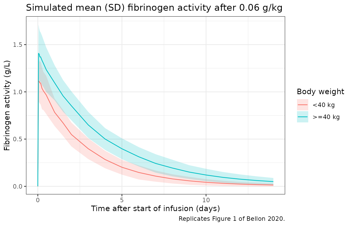
Visual predictive check
Replicates the layout of Figure 2 of Bellon 2020 (5th, 50th and 95th percentiles, stratified by body weight).
sim |>
  dplyr::filter(time > 0) |>
  dplyr::group_by(arm, time) |>
  dplyr::summarise(q05 = quantile(sim, 0.05), q50 = quantile(sim, 0.5),
                   q95 = quantile(sim, 0.95), .groups = "drop") |>
  ggplot(aes(time / 24)) +
  geom_ribbon(aes(ymin = q05, ymax = q95), fill = "grey70", alpha = 0.6) +
  geom_line(aes(y = q50)) +
  facet_wrap(~arm) +
  scale_y_log10() +
  labs(x = "Time after start of infusion (days)",
       y = "Fibrinogen activity (g/L)",
       title = "Simulated 5th-50th-95th percentiles",
       caption = "Replicates Figure 2 of Bellon 2020 (panels A and B).") +
  theme_bw()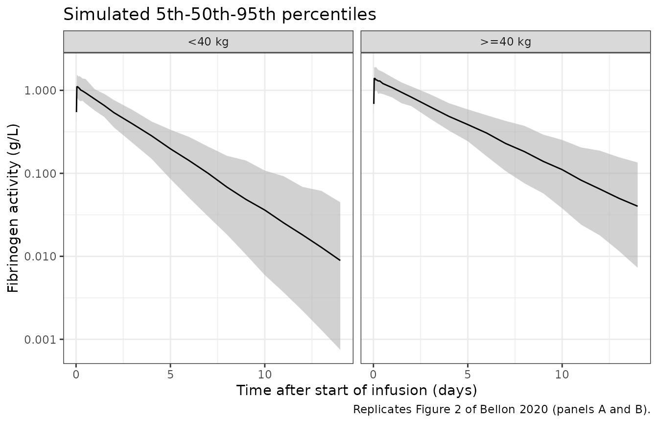
PKNCA validation
NCA is run on the model-predicted concentration Cc
(individual predictions without residual error), which corresponds to
the paper’s Table 4 values derived from individual Bayes estimates. Cmax
is taken at the end of the 1 h infusion, as in the paper (Tmax
“considered the end of infusion”).
conc <- sim |>
  dplyr::filter(!is.na(Cc)) |>
  dplyr::mutate(Cc = pmax(Cc, 0)) |>
  dplyr::select(id, time, Cc, arm)

dose_df <- events |>
  dplyr::filter(evid == 1) |>
  dplyr::mutate(duration = amt / rate) |>
  dplyr::select(id, time, amt, duration, arm)

conc_obj <- PKNCA::PKNCAconc(conc, Cc ~ time | arm + id)
dose_obj <- PKNCA::PKNCAdose(dose_df, amt ~ time | arm + id,
                             duration = "duration", route = "intravascular")
intervals <- data.frame(start = 0, end = Inf, cmax = TRUE, tmax = TRUE,
                        aucinf.obs = TRUE, half.life = TRUE)
nca <- PKNCA::pk.nca(PKNCA::PKNCAdata(conc_obj, dose_obj, intervals = intervals))
nca_res <- as.data.frame(nca$result)
Comparison against the published values
Table 4 of Bellon 2020 reports geometric means of
the individual estimates, so the simulated per-subject NCA results are
summarised with geometric means before the comparison
(ncaComparisonTable() would otherwise pool by the
median).
gmean <- function(x) exp(mean(log(x)))

sim_wide <- nca_res |>
  dplyr::filter(PPTESTCD %in% c("cmax", "aucinf.obs", "half.life")) |>
  dplyr::group_by(arm, PPTESTCD) |>
  dplyr::summarise(PPORRES = gmean(PPORRES), .groups = "drop")

# Bellon 2020 Table 4, fibrinogen activity columns.
ref_wide <- data.frame(
  arm = c("<40 kg", ">=40 kg"),
  cmax = c(1.11, 1.39),
  aucinf.obs = c(81.3, 133.4),
  half.life = c(49.0, 66.7)
)

cmp <- nlmixr2lib::ncaComparisonTable(
  sim_wide, ref_wide, by = "arm",
  units = c(cmax = "g/L", aucinf.obs = "g*h/L", half.life = "h")
)
knitr::kable(cmp)| NCA parameter | arm | Reference | Simulated | % diff |
|---|---|---|---|---|
| Cmax (g/L) | <40 kg | 1.11 | 1.11 | -0.2% |
| Cmax (g/L) | >=40 kg | 1.39 | 1.39 | +0.1% |
| AUC0-∞ (obs) (g*h/L) | <40 kg | 81.3 | 77.5 | -4.7% |
| AUC0-∞ (obs) (g*h/L) | >=40 kg | 133 | 133 | -0.2% |
| t½ (h) | <40 kg | 49 | 48.1 | -1.8% |
| t½ (h) | >=40 kg | 66.7 | 66 | -1.1% |
# Weight-normalised clearance, volume and incremental recovery, compared
# with Table 4 (activity columns). Individual CL and V come from the solve.
indiv <- sim |>
  dplyr::group_by(id, arm) |>
  dplyr::summarise(WT = dplyr::first(WT), cl = dplyr::first(cl),
                   vc = dplyr::first(vc), .groups = "drop") |>
  dplyr::left_join(
    nca_res |> dplyr::filter(PPTESTCD == "cmax") |>
      dplyr::select(id, cmax = PPORRES),
    by = "id"
  ) |>
  dplyr::mutate(cl_kg = 1000 * cl / WT, v_kg = 1000 * vc / WT,
                ir = cmax / 0.06)

per_kg <- indiv |>
  dplyr::group_by(arm) |>
  dplyr::summarise(cl_sim = gmean(cl_kg), v_sim = gmean(v_kg),
                   ir_sim = gmean(ir), .groups = "drop") |>
  dplyr::mutate(cl_ref = c(0.74, 0.45), v_ref = c(52.2, 43.2),
                ir_ref = c(18.5, 23.1))

per_kg |>
  dplyr::select(arm, cl_ref, cl_sim, v_ref, v_sim, ir_ref, ir_sim) |>
  dplyr::rename(
    "Weight group" = arm,
    "CL (mL/h/kg), paper" = cl_ref, "CL (mL/h/kg), simulated" = cl_sim,
    "V (mL/kg), paper" = v_ref, "V (mL/kg), simulated" = v_sim,
    "IR (g/L per g/kg), paper" = ir_ref, "IR (g/L per g/kg), simulated" = ir_sim
  ) |>
knitr::kable(digits = 2)| Weight group | CL (mL/h/kg), paper | CL (mL/h/kg), simulated | V (mL/kg), paper | V (mL/kg), simulated | IR (g/L per g/kg), paper | IR (g/L per g/kg), simulated |
|---|---|---|---|---|---|---|
| <40 kg | 0.74 | 0.77 | 52.2 | 53.74 | 18.5 | 18.47 |
| >=40 kg | 0.45 | 0.45 | 43.2 | 42.90 | 23.1 | 23.18 |
# Group-level geometric means over 200 subjects. The between-subject CV is
# about 20-25%, so the Monte-Carlo SE of a 200-subject geometric mean is
# about 1.5-2%; the cohort weight distribution is an approximation of the
# paper's. A mis-transcribed parameter moves these by tens of percent.
nca_check <- ref_wide |>
  tidyr::pivot_longer(-arm, names_to = "PPTESTCD", values_to = "ref") |>
  dplyr::inner_join(sim_wide, by = c("arm", "PPTESTCD"))
stopifnot(
  nrow(nca_check) == 6L,
  all(abs(nca_check$PPORRES / nca_check$ref - 1) < 0.15),
  all(abs(per_kg$cl_sim / per_kg$cl_ref - 1) < 0.15),
  all(abs(per_kg$v_sim / per_kg$v_ref - 1) < 0.15),
  all(abs(per_kg$ir_sim / per_kg$ir_ref - 1) < 0.10)
)
The simulated geometric means reproduce the weight-group results of Table 4: lower Cmax and incremental recovery, higher weight-normalised clearance and a shorter half-life in patients under 40 kg. The paper’s dosing conclusion follows: 1 g/kg raises fibrinogen activity by about 19 g/L under 40 kg and about 23 g/L at or above 40 kg.
Assumptions and deviations
- Antigen model not encoded. The same structural model was fitted to fibrinogen antigen (nephelometry), but only the individual-estimate summaries (Table 4) are published, not the antigen population parameters. Only the activity model is included.
- No endogenous baseline. The patients were afibrinogenaemic, with pre-dose fibrinogen below the assay limit, and the paper’s model has no baseline term. The model therefore should not be used for hypofibrinogenaemic patients with measurable baseline fibrinogen without adding a baseline.
-
Uncentred body weight. The paper uses actual body
weight without centring, so
lclandlvcare the typical values for a 1 kg patient. They are kept in that form so the parameter values match Table 2. - Residual-error equation. Section 3.1 equation 3 (the residual-error model) did not survive into the extractable text. The proportional form comes from sections 2.3.1 and 3.2, and the magnitude is the square root of the Table 2 sigma^2 (0.0120), consistent with its 11.0% CV column.
- Virtual cohort. The individual weights are not published. The simulation draws log-normal weights around the Table 1 medians, truncated to the Table 1 ranges, and uses a fixed 1 h infusion (the median). Race and region are not reported.
- Supplement not reviewed. Supplementary Tables S1 (covariate search) and S2 (PK by study) and Figures S1-S3 (goodness of fit) were not available when this model was added. They hold no model parameters; the final estimates are all in the main-text Table 2.
- No erratum was found in a Europe PMC search on 2026-09-25.