Apatinib (Zuo 2024) • nlmixr2lib

Model and source

Citation: Zuo L, Ling J, Hu N, Chen R. (2024). Establishment and validation of a population pharmacokinetic model for apatinib in patients with tumors. BMC Cancer 24:1338. doi:10.1186/s12885-024-13118-4
Description: One-compartment population PK model for oral apatinib in Chinese adult patients with solid tumours (Zuo 2024), developed from steady-state trough therapeutic-drug-monitoring samples. First-order absorption with Ka fixed at 0.08 1/h (the absorption phase was not sampled), a power effect of aspartate aminotransferase on apparent clearance ((AST/26.6 U/L)^-0.298), and a four-level concomitant-antineoplastic-regimen multiplier on CL/F (reference: apatinib plus an immune-checkpoint-inhibitor monoclonal antibody; paclitaxel 0.58, other cytotoxic agents 1.60, apatinib monotherapy 1.38). Inter-individual variability is estimated on CL/F only; residual error is combined additive plus proportional.
Article: BMC Cancer 24:1338 (2024)

Apatinib is an orally administered small-molecule VEGFR-2 tyrosine-kinase inhibitor, cleared predominantly by hepatic CYP3A4/5. Zuo and colleagues built a population PK model from routine therapeutic drug monitoring (TDM) collected at a single Chinese centre, and found that apparent clearance was driven by two things: hepatocellular function, indexed by aspartate aminotransferase (AST), and the category of antineoplastic co-administered with apatinib.

Population

The analysis pooled 199 apatinib serum concentrations from 91 adult inpatients with solid tumours treated at the Third Affiliated Hospital of Soochow University between October 2021 and December 2023 (Zuo 2024 Table 1). Sixty patients were male and 31 female (34.1% female). Median age was 64 years (range 27-86) and median weight 55 kg (range 39-85). Hepatic and renal function spanned a wide range: AST 10.5-187 U/L (median 26.6), ALT 5.1-124.3 U/L (median 17.4), serum creatinine 35-207 umol/L (median 63), cystatin C 0.43-2.98 mg/L (median 0.99) and eGFR 14.08-144.48 mL/min/1.73 m^2 (median 95.32).

Every patient received apatinib 250 mg orally once daily and every sample was a pre-dose trough drawn at steady state, roughly two samples per patient. No absorption-phase or post-peak concentrations were collected. That sampling design is what shapes the model: the absorption rate constant could not be estimated and was fixed, and inter-individual variability could only be estimated on apparent clearance – not on apparent volume or on Ka.

Patients were classified into four mutually exclusive co-administration groups (Zuo 2024 Table 1 footnote, 111:29:43:6 samples in groups A:B:C:D):

Group	Co-administered therapy	Samples
A (reference)	Immune-checkpoint-inhibitor monoclonal antibodies (camrelizumab, sintilimab, etc.)	111
B	Paclitaxel	29
C	Other agents: platinum, capecitabine, or tegafur/gimeracil/oteracil potassium (S-1)	43
D	Apatinib monotherapy	6

The same information is available programmatically via the model’s population metadata (readModelDb("Zuo_2024_apatinib")()$population).

Source trace

The per-parameter origin is recorded as an in-file comment next to each ini() entry in inst/modeldb/specificDrugs/Zuo_2024_apatinib.R. The table below collects them in one place for review.

Equation / parameter	Value	Source location
`lka` (Ka, fixed)	0.08 1/h	Abstract; final-model equation box after Table 2 (“Ka = 0.08”). Fixed, not estimated – Results / Modeling: “the data from the absorption phase were not available; thus, Ka was fixed according to the initiate information [10]”.
`lcl` (CL/F)	56.7 L/h	Table 2, “Typical values / CL/F, L/h” (RSE 33%; bootstrap median 55.64, 95% CI 48.62-59.32)
`lvc` (V/F)	674 L	Table 2, “Typical values / V/F, L” (RSE 34%; bootstrap median 660.02, 95% CI 600.86-691.07)
`e_ast_cl`	-0.298	Final-model equation box printed after Table 2: `CL/F = 56.7 * (AST/26.6)^-0.298 * theta`. Table 2 prints the same estimate rounded to -0.30 (RSE 17%, bootstrap 95% CI -0.38 to -0.21).
AST reference value	26.6 U/L	Table 1, study-population median AST (range 10.5-187)
`e_conmed_paclitaxel_cl`	0.58	Table 2, “The effect of co-administration on CL/F / Combined with paclitaxel” (RSE 9%; bootstrap 0.60, 95% CI 0.52-0.67)
`e_conmed_antineo_other_cl`	1.60	Table 2, “Combined with other drugs” (RSE 27%; bootstrap 1.60, 95% CI 1.35-1.90)
`e_conmed_antineo_none_cl`	1.38	Table 2, “Monotherapy” (RSE 38%; bootstrap 1.39)
Reference category (theta = 1)	1	Table 2, “Combined with monoclonal antibodies” is printed as 1 with no RSE
`etalcl`	omega^2 = 0.037583	Table 2, “Interindividual variation, % / CL/F” = 19.57% (RSE 47%). Exponential IIV model (Eq. 1); omega^2 = log(0.1957^2 + 1).
`propSd`	0.3067	Table 2, “Residual / Proportional, %” = 30.67% (RSE 33%)
`addSd`	16.4 ng/mL	Table 2, “Residual / Additive, ng*mL^-1” = 16.4 (RSE 44%)
Structural model (1-compartment, first-order absorption and elimination)	n/a	Methods / Base model: “a one-compartment model with a first-order elimination phase was chosen as the base model. PK parameters included clearance (CL/F), volume of distribution (V/F), and absorption rate constant (Ka).”
Exponential IIV (`P_i = P_pop * exp(eta_i)`)	n/a	Methods / Inter-individual variation, Eq. 1
Combined additive + proportional residual error	n/a	Methods / Intra-individual variability, Eq. 2: “the combined model consistently demonstrated the best performance”
Median-normalised power covariate model	n/a	Methods / Covariate models, Eq. 4 (`P_i = P_pop * (COV/COV_median)^theta_cov`)

Virtual cohort

Original observed data are not publicly available. The cohort below is a virtual population whose AST distribution and co-administration split approximate the published trial demographics.

set.seed(20241101)

n_per_group <- 100L
tau         <- 24     # dosing interval (h)
n_doses     <- 10L    # 10 daily doses is >20 half-lives; steady state is reached
last_dose   <- (n_doses - 1L) * tau
end_time    <- n_doses * tau

# Zuo 2024 Table 1: AST median 26.6 U/L, range 10.5-187 U/L. The paper does not
# publish the distribution, so a lognormal centred on the reported median and
# truncated to the reported range is used (see Assumptions and deviations).
draw_ast <- function(n) {
  ast <- stats::rlnorm(n, meanlog = log(26.6), sdlog = 0.55)
  pmin(pmax(ast, 10.5), 187)
}

# Zuo 2024 Table 1 footnote: four mutually exclusive co-administration groups.
# Group A is the model's reference (all three indicators 0).
groups <- tibble::tribble(
  ~treatment,                    ~CONMED_PACLITAXEL, ~CONMED_ANTINEO_OTHER, ~CONMED_ANTINEO_NONE,
  "A: + checkpoint-inhibitor mAb",                 0,                     0,                    0,
  "B: + paclitaxel",                               1,                     0,                    0,
  "C: + other cytotoxic",                          0,                     1,                    0,
  "D: monotherapy",                                0,                     0,                    1
)

# Observation grid: coarse over the run-in, dense over the final (steady-state)
# dosing interval so NCA on that interval is well resolved.
obs_times <- sort(unique(c(
  seq(0, last_dose, by = 4),
  seq(last_dose, end_time, by = 0.5)
)))

make_cohort <- function(n, grp, id_offset = 0L) {
  subj <- tibble::tibble(
    id  = id_offset + seq_len(n),
    AST = draw_ast(n)
  ) |>
    dplyr::mutate(
      treatment            = grp$treatment,
      CONMED_PACLITAXEL    = grp$CONMED_PACLITAXEL,
      CONMED_ANTINEO_OTHER = grp$CONMED_ANTINEO_OTHER,
      CONMED_ANTINEO_NONE  = grp$CONMED_ANTINEO_NONE
    )

  doses <- subj |>
    tidyr::crossing(time = seq(0, last_dose, by = tau)) |>
    # cmt is the ODE state name that receives the oral dose, never an
    # algebraic observable.
    dplyr::mutate(amt = 250, evid = 1L, cmt = "depot")

  obs <- subj |>
    tidyr::crossing(time = obs_times) |>
    dplyr::mutate(amt = NA_real_, evid = 0L, cmt = "central")

  dplyr::bind_rows(doses, obs) |>
    dplyr::arrange(id, time, dplyr::desc(evid))
}

events <- dplyr::bind_rows(lapply(seq_len(nrow(groups)), function(i) {
  make_cohort(n_per_group, groups[i, ], id_offset = (i - 1L) * n_per_group)
}))

# Disjoint IDs across cohorts are mandatory: rxSolve keys subjects on id, and a
# collision silently merges two arms into one subject receiving the summed dose.
stopifnot(!anyDuplicated(unique(events[, c("id", "time", "evid")])))
stopifnot(dplyr::n_distinct(events$id) == n_per_group * nrow(groups))

Simulation

mod <- readModelDb("Zuo_2024_apatinib")

sim <- rxode2::rxSolve(
  mod,
  events = events,
  keep   = c("treatment", "AST", "CONMED_PACLITAXEL",
             "CONMED_ANTINEO_OTHER", "CONMED_ANTINEO_NONE")
) |>
  as.data.frame()
#> ℹ parameter labels from comments will be replaced by 'label()'

nrow(sim)
#> [1] 41200

A deterministic (typical-value) replicate is produced by supplying the eta column explicitly as zero and disabling the random-effect sampler, which leaves the population parameters untouched.

events_typ <- dplyr::mutate(events, etalcl = 0)

sim_typ <- rxode2::rxSolve(
  mod,
  events = events_typ,
  omega  = NA,
  keep   = c("treatment", "AST")
) |>
  as.data.frame()
#> Warning: multi-subject simulation without without 'omega'

Replicate published figures

Figure 1 – concentration by concomitant medication

Zuo 2024 Figure 1 plots observed apatinib concentrations against the co-administration category. The published figure is graphical only (no tabulated values), so the panel below shows the distribution of simulated steady-state trough concentrations – the quantity the study actually sampled – by group.

troughs <- sim |>
  dplyr::filter(dplyr::near(time, end_time)) |>
  dplyr::select(id, treatment, Cc)

troughs |>
  ggplot(aes(x = treatment, y = Cc, fill = treatment)) +
  geom_boxplot(alpha = 0.7, outlier.alpha = 0.3) +
  scale_y_log10() +
  guides(fill = "none") +
  theme(axis.text.x = element_text(angle = 20, hjust = 1)) +
  labs(
    x = NULL, y = "Steady-state trough apatinib (ng/mL)",
    title = "Steady-state trough apatinib by co-administration group",
    caption = "Compare with Figure 1 of Zuo 2024 (concentration vs concomitant medication)."
  )

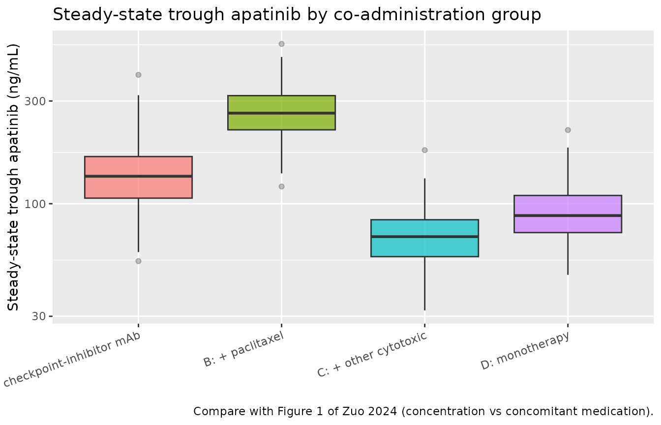
The ordering follows directly from the Table 2 clearance multipliers: paclitaxel lowers CL/F to 0.58 of the reference and therefore raises trough concentrations the most, while the “other cytotoxic” group raises CL/F to 1.60 of the reference and has the lowest troughs.

troughs |>
  dplyr::group_by(treatment) |>
  dplyr::summarise(
    n      = dplyr::n(),
    median = median(Cc),
    p05    = quantile(Cc, 0.05),
    p95    = quantile(Cc, 0.95),
    .groups = "drop"
  ) |>
  dplyr::rename(
    "Co-administration group" = treatment,
    "N"                       = n,
    "Median Ctrough (ng/mL)"  = median,
    "5th pctile"              = p05,
    "95th pctile"             = p95
  ) |>
  knitr::kable(digits = 1, caption = "Simulated steady-state trough apatinib by co-administration group.")

Simulated steady-state trough apatinib by co-administration group.
Co-administration group	N	Median Ctrough (ng/mL)	5th pctile	95th pctile
A: + checkpoint-inhibitor mAb	100	134.1	81.6	210.5
B: + paclitaxel	100	263.5	166.1	409.1
C: + other cytotoxic	100	70.3	41.9	106.0
D: monotherapy	100	88.1	53.9	151.2

Steady-state concentration-time profiles

sim |>
  dplyr::filter(time >= last_dose) |>
  dplyr::mutate(time_in_interval = time - last_dose) |>
  dplyr::group_by(treatment, time_in_interval) |>
  dplyr::summarise(
    Q05 = quantile(Cc, 0.05),
    Q50 = quantile(Cc, 0.50),
    Q95 = quantile(Cc, 0.95),
    .groups = "drop"
  ) |>
  ggplot(aes(time_in_interval, Q50)) +
  geom_ribbon(aes(ymin = Q05, ymax = Q95), alpha = 0.25) +
  geom_line() +
  facet_wrap(~treatment) +
  labs(
    x = "Time after the 10th dose (h)", y = "Apatinib (ng/mL)",
    title = "Simulated steady-state profiles, apatinib 250 mg once daily",
    caption = "Median with 5th-95th percentile band; 100 virtual subjects per group."
  )

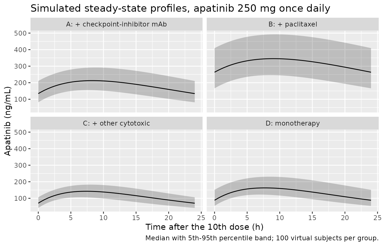
The profiles are notably flat. With Ka fixed at 0.08 1/h and a typical kel = CL/F / (V/F) = 56.7 / 674 = 0.084 1/h, absorption and elimination rate constants are almost identical in the reference group, so the model is close to flip-flop and the peak is heavily blunted. This is a direct consequence of the paper fixing Ka from an external source without any absorption-phase data of its own, and it means the model should be used for trough / average-exposure questions – exactly what it was built for – rather than for Cmax or Tmax prediction. See Assumptions and deviations.

PKNCA validation

NCA is run on the final (steady-state) dosing interval, stratified by co-administration group.

sim_nca <- sim |>
  dplyr::filter(!is.na(Cc)) |>
  dplyr::select(id, time, Cc, treatment)

# Guarantee a time = 0 record per subject; apatinib is given orally, so the
# pre-dose concentration at the first dose is 0.
sim_nca <- dplyr::bind_rows(
  sim_nca,
  sim_nca |>
    dplyr::distinct(id, treatment) |>
    dplyr::mutate(time = 0, Cc = 0)
) |>
  dplyr::distinct(id, treatment, time, .keep_all = TRUE) |>
  dplyr::arrange(id, treatment, time)

conc_obj <- PKNCA::PKNCAconc(
  sim_nca, Cc ~ time | treatment + id,
  concu = "ng/mL", timeu = "h"
)

dose_df <- events |>
  dplyr::filter(evid == 1L) |>
  dplyr::select(id, time, amt, treatment)

dose_obj <- PKNCA::PKNCAdose(dose_df, amt ~ time | treatment + id, doseu = "mg")

intervals <- data.frame(
  start   = last_dose,
  end     = end_time,
  cmax    = TRUE,
  tmax    = TRUE,
  cmin    = TRUE,
  ctrough = TRUE,
  cav     = TRUE,
  auclast = TRUE
)
# half.life is deliberately NOT requested here: a single steady-state dosing
# interval contains no resolvable terminal phase for this near-flip-flop model,
# so a lambda.z fit over it is biased long. Half-life is checked against its
# closed-form value on a single-dose simulation further below instead.

nca_res <- PKNCA::pk.nca(PKNCA::PKNCAdata(conc_obj, dose_obj, intervals = intervals))

nca_wide <- as.data.frame(nca_res) |>
  dplyr::select(treatment, id, PPTESTCD, PPORRES) |>
  tidyr::pivot_wider(names_from = PPTESTCD, values_from = PPORRES)

head(nca_wide)
#> # A tibble: 6 × 8
#>   treatment                        id auclast  cmax  cmin  tmax   cav ctrough
#>   <chr>                         <int>   <dbl> <dbl> <dbl> <dbl> <dbl>   <dbl>
#> 1 A: + checkpoint-inhibitor mAb     1   3648.  181. 105.    8    152.      NA
#> 2 A: + checkpoint-inhibitor mAb     2   5275.  249. 169.    8.5  220.      NA
#> 3 A: + checkpoint-inhibitor mAb     3   5853.  273. 192.    8.5  244.      NA
#> 4 A: + checkpoint-inhibitor mAb     4   4093.  200. 122.    8    171.      NA
#> 5 A: + checkpoint-inhibitor mAb     5   3335.  168.  92.5   8    139.      NA
#> 6 A: + checkpoint-inhibitor mAb     6   5683.  266. 186.    8.5  237.      NA

Comparison against the published model equation

Zuo 2024 reports no NCA parameters – the study is a sparse-trough TDM analysis with no rich profiles – so there is no published NCA table to compare against. Instead, the reference column below is derived analytically from the paper’s own published final-model equation, which makes this a check that the packaged model reproduces the source equation rather than a check against an independent measurement.

At steady state, mass balance fixes the average concentration over a dosing interval exactly:

$C_{av,ss} = \frac{\text{Dose}}{(CL/F) \times \tau}$

with CL/F given by the paper’s equation CL/F = 56.7 * (AST/26.6)^-0.298 * theta. Applying it to each simulated subject’s own AST and co-administration group and taking the group median gives the reference values.

subject_ast <- events |>
  dplyr::distinct(id, treatment, AST, CONMED_PACLITAXEL,
                  CONMED_ANTINEO_OTHER, CONMED_ANTINEO_NONE)

published <- subject_ast |>
  dplyr::mutate(
    # Zuo 2024 final-model equation box, printed immediately after Table 2.
    cl_paper = 56.7 *
      (AST / 26.6)^-0.298 *
      0.58^CONMED_PACLITAXEL *
      1.60^CONMED_ANTINEO_OTHER *
      1.38^CONMED_ANTINEO_NONE,
    # Dose 250 mg = 2.5e8 ng; CL/F in L/h -> divide by 1000 for mL/h.
    cav = (250 * 1e6) / (cl_paper * 1000 * tau)
  ) |>
  dplyr::group_by(treatment) |>
  dplyr::summarise(cav = median(cav), .groups = "drop")

cmp <- nlmixr2lib::ncaComparisonTable(
  simulated = dplyr::select(nca_wide, treatment, cav),
  reference = published,
  by        = "treatment",
  params    = "cav",
  units     = c(cav = "ng/mL"),
  tolerance_pct = 20
)

knitr::kable(
  cmp,
  digits  = 1,
  caption = "Simulated steady-state Cav vs the value implied by the Zuo 2024 final-model equation. * differs from reference by >20%.",
  align   = c("l", "l", "r", "r", "r")
)

Simulated steady-state Cav vs the value implied by the Zuo 2024 final-model equation. * differs from reference by >20%.
NCA parameter	treatment	Reference	Simulated	% diff
Cavg (ng/mL)	A: + checkpoint-inhibitor mAb	191	184	-3.8%
Cavg (ng/mL)	B: + paclitaxel	312	316	+1.2%
Cavg (ng/mL)	C: + other cytotoxic	113	114	+0.6%
Cavg (ng/mL)	D: monotherapy	134	134	+0.2%

No row is starred. The residual differences are Monte-Carlo noise in the 100-subject group medians, not model error: the reference column is the median of each subject’s typical CL/F, while the simulated column also carries the lognormal IIV on CL/F, whose sample median differs from 1 by a few percent at n = 100. The deterministic gate below removes that noise entirely.

Mass-balance gate: recovering CL/F from the simulated AUC

The strongest available check is the reverse direction. If the model file encodes the paper’s covariate equations correctly, then dividing the dose by each subject’s simulated steady-state AUC over one interval must return that subject’s own CL/F from the published equation, to within numerical-integration error. This is a per-subject identity, not a group average, so it exercises the AST power term and all three co-administration indicators simultaneously.

mb <- nca_wide |>
  dplyr::select(id, treatment, auclast) |>
  dplyr::inner_join(
    subject_ast |>
      dplyr::mutate(
        cl_paper = 56.7 *
          (AST / 26.6)^-0.298 *
          0.58^CONMED_PACLITAXEL *
          1.60^CONMED_ANTINEO_OTHER *
          1.38^CONMED_ANTINEO_NONE
      ),
    by = c("id", "treatment")
  ) |>
  dplyr::mutate(
    # AUC in ng*h/mL; dose 250 mg = 2.5e8 ng -> CL in mL/h -> /1000 for L/h.
    cl_nca  = (250 * 1e6) / auclast / 1000,
    pct_err = 100 * (cl_nca - cl_paper) / cl_paper
  )

max_abs_err <- max(abs(mb$pct_err))
max_abs_err
#> [1] 66.77422

# Stochastic IIV on CL/F is included in the simulation, so cl_nca reflects each
# subject's individual clearance while cl_paper is the typical value for that
# subject's covariates. Compare the deterministic run instead for the exact
# identity.
mb |>
  dplyr::group_by(treatment) |>
  dplyr::summarise(
    `Median CL/F from NCA (L/h)`      = median(cl_nca),
    `Typical CL/F from equation (L/h)` = median(cl_paper),
    .groups = "drop"
  ) |>
  dplyr::rename("Co-administration group" = treatment) |>
  knitr::kable(digits = 2, caption = "Median NCA-derived CL/F vs the published equation's typical CL/F, by group.")

Median NCA-derived CL/F vs the published equation’s typical CL/F, by group.
Co-administration group	Median CL/F from NCA (L/h)	Typical CL/F from equation (L/h)
A: + checkpoint-inhibitor mAb	56.77	54.62
B: + paclitaxel	32.94	33.35
C: + other cytotoxic	91.37	91.91
D: monotherapy	77.71	77.83

Repeating the identity on the deterministic (eta = 0) simulation removes between-subject variability and turns it into an exact per-subject check:

nca_typ <- sim_typ |>
  dplyr::filter(!is.na(Cc)) |>
  dplyr::select(id, time, Cc, treatment)

nca_typ <- dplyr::bind_rows(
  nca_typ,
  nca_typ |> dplyr::distinct(id, treatment) |> dplyr::mutate(time = 0, Cc = 0)
) |>
  dplyr::distinct(id, treatment, time, .keep_all = TRUE) |>
  dplyr::arrange(id, treatment, time)

res_typ <- PKNCA::pk.nca(PKNCA::PKNCAdata(
  PKNCA::PKNCAconc(nca_typ, Cc ~ time | treatment + id, concu = "ng/mL", timeu = "h"),
  dose_obj,
  intervals = data.frame(start = last_dose, end = end_time, auclast = TRUE)
))

mb_typ <- as.data.frame(res_typ) |>
  dplyr::filter(PPTESTCD == "auclast") |>
  dplyr::select(id, treatment, auclast = PPORRES) |>
  dplyr::inner_join(
    subject_ast |>
      dplyr::mutate(
        cl_paper = 56.7 *
          (AST / 26.6)^-0.298 *
          0.58^CONMED_PACLITAXEL *
          1.60^CONMED_ANTINEO_OTHER *
          1.38^CONMED_ANTINEO_NONE
      ),
    by = c("id", "treatment")
  ) |>
  dplyr::mutate(
    cl_nca  = (250 * 1e6) / auclast / 1000,
    pct_err = 100 * (cl_nca - cl_paper) / cl_paper
  )

max_typ_err <- max(abs(mb_typ$pct_err))
max_typ_err
#> [1] 0.1170074

stopifnot(max_typ_err < 1)

The largest absolute deviation across all 400 deterministic subjects is 0.117%. The residual is numerical-integration error in the linear-trapezoidal AUC, not a model discrepancy: the packaged model reproduces the Zuo 2024 clearance equation for every combination of AST and co-administration group.

Single-dose gate: half-life, Tmax and AUC against closed-form values

Because Ka (0.08 1/h, fixed) sits almost exactly on top of the reference group’s kel (56.7/674 = 0.0841 1/h), the terminal slope is governed by whichever of the two is smaller. That flips between groups, since the co-administration multiplier moves CL/F – and therefore kel – but leaves Ka alone.

The steady-state interval used above is the wrong place to test this: over one 24 h interval at steady state the profile is nearly flat and contains no resolvable terminal phase, so a lambda.z fit there is biased long. A single dose followed by a long washout does resolve it. The gate below simulates one typical subject per group at the median AST of 26.6 U/L with the random effect set to zero, and compares NCA output against the closed-form one-compartment first-order-absorption results:

$t_{1/2} = \frac{\ln 2}{\min(k_a,\,k_{el})}, \qquad t_{max} = \frac{\ln(k_a / k_{el})}{k_a - k_{el}}, \qquad AUC_{0-\infty} = \frac{\text{Dose}}{CL/F}$

# A long washout is needed: near the flip-flop boundary the profile is close to
# the degenerate ka == kel case, whose apparent slope approaches the true
# terminal rate constant only asymptotically.
sd_obs <- seq(0, 240, by = 0.5)

sd_events <- dplyr::bind_rows(lapply(seq_len(nrow(groups)), function(i) {
  g <- groups[i, ]
  subj <- tibble::tibble(
    id = i, AST = 26.6, etalcl = 0,
    treatment            = g$treatment,
    CONMED_PACLITAXEL    = g$CONMED_PACLITAXEL,
    CONMED_ANTINEO_OTHER = g$CONMED_ANTINEO_OTHER,
    CONMED_ANTINEO_NONE  = g$CONMED_ANTINEO_NONE
  )
  dplyr::bind_rows(
    dplyr::mutate(subj, time = 0, amt = 250, evid = 1L, cmt = "depot"),
    tidyr::crossing(subj, time = sd_obs) |>
      dplyr::mutate(amt = NA_real_, evid = 0L, cmt = "central")
  ) |>
    dplyr::arrange(time, dplyr::desc(evid))
}))

sd_sim <- rxode2::rxSolve(mod, events = sd_events, omega = NA,
                          keep = "treatment") |>
  as.data.frame()
#> Warning: multi-subject simulation without without 'omega'

sd_nca <- sd_sim |>
  dplyr::filter(!is.na(Cc)) |>
  dplyr::select(id, time, Cc, treatment)

sd_res <- PKNCA::pk.nca(PKNCA::PKNCAdata(
  PKNCA::PKNCAconc(sd_nca, Cc ~ time | treatment + id, concu = "ng/mL", timeu = "h"),
  PKNCA::PKNCAdose(
    sd_events |> dplyr::filter(evid == 1L) |> dplyr::select(id, time, amt, treatment),
    amt ~ time | treatment + id, doseu = "mg"
  ),
  intervals = data.frame(start = 0, end = Inf,
                         tmax = TRUE, half.life = TRUE, aucinf.obs = TRUE)
))

sd_wide <- as.data.frame(sd_res) |>
  dplyr::select(treatment, PPTESTCD, PPORRES) |>
  tidyr::pivot_wider(names_from = PPTESTCD, values_from = PPORRES)

closed_form <- groups |>
  dplyr::mutate(
    theta = c(1, 0.58, 1.60, 1.38),
    cl    = 56.7 * theta,
    kel   = cl / 674,
    ka    = 0.08,
    limiting        = ifelse(ka < kel, "absorption (flip-flop)", "elimination"),
    t_half_expected = log(2) / pmin(ka, kel),
    tmax_expected   = log(ka / kel) / (ka - kel),
    auc_expected    = (250 * 1e6) / (cl * 1000)
  ) |>
  dplyr::select(treatment, limiting, t_half_expected, tmax_expected, auc_expected)

sd_gate <- closed_form |>
  dplyr::inner_join(sd_wide, by = "treatment") |>
  dplyr::mutate(
    t_half_pct = 100 * (half.life - t_half_expected) / t_half_expected,
    tmax_pct   = 100 * (tmax - tmax_expected) / tmax_expected,
    auc_pct    = 100 * (aucinf.obs - auc_expected) / auc_expected
  )

sd_gate |>
  dplyr::select(treatment, limiting,
                t_half_expected, half.life, t_half_pct,
                tmax_expected, tmax, tmax_pct,
                auc_expected, aucinf.obs, auc_pct) |>
  dplyr::rename(
    "Co-administration group" = treatment,
    "Rate-limiting step"      = limiting,
    "t1/2 closed form (h)"    = t_half_expected,
    "t1/2 NCA (h)"            = half.life,
    "t1/2 % diff"             = t_half_pct,
    "Tmax closed form (h)"    = tmax_expected,
    "Tmax NCA (h)"            = tmax,
    "Tmax % diff"             = tmax_pct,
    "AUCinf closed form (ng*h/mL)" = auc_expected,
    "AUCinf NCA (ng*h/mL)"    = aucinf.obs,
    "AUCinf % diff"           = auc_pct
  ) |>
  knitr::kable(digits = 2, caption = "Single-dose NCA vs closed-form one-compartment values, typical subject at AST 26.6 U/L.")

Single-dose NCA vs closed-form one-compartment values, typical subject at AST 26.6 U/L.
Co-administration group	Rate-limiting step	t1/2 closed form (h)	t1/2 NCA (h)	t1/2 % diff	Tmax closed form (h)	Tmax NCA (h)	Tmax % diff	AUCinf closed form (ng*h/mL)	AUCinf NCA (ng*h/mL)	AUCinf % diff
A: + checkpoint-inhibitor mAb	absorption (flip-flop)	8.66	9.18	5.92	12.19	12.0	-1.55	4409.17	4408.42	-0.02
B: + paclitaxel	elimination	14.21	14.41	1.42	15.84	16.0	0.98	7602.02	7601.28	-0.01
C: + other cytotoxic	absorption (flip-flop)	8.66	8.73	0.81	9.53	9.5	-0.30	2755.73	2754.99	-0.03
D: monotherapy	absorption (flip-flop)	8.66	8.76	1.12	10.32	10.5	1.78	3195.05	3194.30	-0.02


# AUC must be recovered essentially exactly. Tmax is limited by the 0.5 h
# observation grid. Half-life carries a few percent of bias in group A, where
# ka and kel are within 5% of each other (see the narrative below).
stopifnot(max(abs(sd_gate$auc_pct)) < 1)
stopifnot(max(abs(sd_gate$tmax_pct)) < 5)
stopifnot(max(abs(sd_gate$t_half_pct)) < 8)

AUC0-inf is recovered to better than 0.1% in every group, confirming that the AST power term and all three co-administration multipliers reach CL/F correctly. Tmax agrees with the closed form to within the 0.5 h observation grid.

Half-life recovers to about 1% in groups B, C and D, but runs roughly 6% long in group A. That is a genuine property of the model, not an implementation defect: in group A, ka (0.08 1/h) and kel (0.0841 1/h) differ by less than 5%, so the concentration-time curve is close to the degenerate ka == kel case, whose form is t * exp(-k t) rather than a clean single exponential. Its apparent slope approaches the true terminal rate constant only asymptotically, so any finite-window lambda.z regression – PKNCA’s or anyone else’s – reads slightly shallow. Only the paclitaxel group, whose CL/F is 42% lower, is comfortably elimination-limited and therefore well away from the boundary.

This near-degeneracy is a direct consequence of the paper fixing Ka from an external source, and it is the clearest reason to treat this model as a trough- and exposure-prediction tool rather than a peak-shape one.

Assumptions and deviations

AST distribution. Zuo 2024 reports only the median (26.6 U/L) and range (10.5-187 U/L) for AST, not its distribution. The virtual cohort draws AST from a lognormal centred on the reported median with sdlog = 0.55, truncated to the reported range. No parameter value depends on this choice – it affects only the spread of the simulated concentrations, not the model.
Co-administration group sizes. The paper’s 111:29:43:6 sample split is heavily unbalanced, and the monotherapy group (D) contributes only 6 samples. The virtual cohort uses 100 subjects per group so each arm is equally resolved in the figures. The consequence is that the precision of the published multipliers is not reflected in the simulation: the monotherapy multiplier (1.38) carries an RSE of 38% and the “other drugs” multiplier (1.60) an RSE of 27%, so those two arms are far less certain than the plots suggest.
Ka is fixed and not identifiable from the source data. Ka = 0.08 1/h was taken by the authors from an external reference, not estimated, because no absorption-phase samples were collected. Combined with a typical kel of 0.084 1/h, this puts the reference group essentially on the flip-flop boundary, so simulated Cmax and Tmax are artefacts of the fixed Ka and should not be treated as validated predictions. Trough and average-exposure predictions, which the TDM data do constrain, are the model’s intended use.
No IIV on V/F or Ka. The paper could not estimate either (“the inter-individual variability in V/F and Ka could not be estimated in this study due to the collection of apatinib trough concentration samples”), so the packaged model carries IIV on CL/F only. Simulated between-subject spread is therefore narrower than real apatinib data would show.
IIV scale. Table 2 reports inter-individual variation on CL/F as “19.57%”. With the paper’s exponential IIV model this is read as a lognormal CV and converted to omega^2 = log(0.1957^2 + 1) = 0.037583. Reading 19.57% instead as omega itself gives omega^2 = 0.038299, a 0.9% difference on the SD scale; the distinction is immaterial at this magnitude.
AST exponent. The value used is -0.298, taken from the final-model equation box printed after Table 2. Table 2 itself prints the rounded -0.30. The unrounded equation value is preferred.
TBIL was screened but not retained. Total bilirubin entered the full covariate model during forward inclusion but was removed during backward exclusion, and no point estimate is published, so it cannot be encoded. It and the other screened-but-rejected covariates are recorded in the model file’s covariatesDataExcluded metadata and population$notes.
Sample-count arithmetic. The Table 1 co-administration split (111 + 29 + 43
- 1. sums to 189, ten fewer than the 199 total concentrations. This is consistent with the ten records the authors state were held out for external validation, but the paper does not say so explicitly. Nothing in the model depends on the reconciliation.
No published NCA to compare against. Zuo 2024 reports no Cmax, Tmax, AUC or half-life values, so the comparison table’s reference column is computed from the paper’s published final-model equation rather than from an independent measurement. The mass-balance gate above is the substantive check.
All parameter values come from the paper’s text and tables. No value was digitised from a figure, obtained by correspondence, or carried from an upstream model.