Anti-CD4 trimeric nanobody and ibalizumab in HIV-1 (Fan 2025)
Source:vignettes/articles/Fan_2025_antiCD4_nanobody_HIV.Rmd
Fan_2025_antiCD4_nanobody_HIV.RmdModels and source
Fan 2025 develops one mechanism-based quasi-equilibrium (QE) target-mediated drug disposition (TMDD) PK model coupled to an HIV-1 viral-dynamic PD model, fits it separately to two drugs in HIV-1-infected humanized mice, and then scales each fit to humans by allometry. That is four self-contained models, so this paper contributes four files and this single vignette.
| Model | Species | Disposition | Role in the paper |
|---|---|---|---|
Fan_2025_nb457trimer_mouse |
mouse | 1-compartment | The fitted nanobody model (Table 1 / Table 2, Nb457 rows) |
Fan_2025_ibalizumab_mouse |
mouse | 2-compartment | The fitted positive-control model (Table 1 / Table 2, Ibalizumab rows) |
Fan_2025_nb457trimer_human |
human | 1-compartment | Allometric projection used for Fig. 4 and Fig. 5 |
Fan_2025_ibalizumab_human |
human | 2-compartment | Allometric projection validated against clinical PK (Fig. S7, S8) |
- Citation: Fan X, Cao K, Wu X, Yan X. Pharmacokinetic-pharmacodynamic modeling of a highly potent and broadly neutralizing anti-CD4 trimeric nanobody to inhibit HIV-1 infection. Microbiol Spectr. 2025;13(11):e00805-25. doi:10.1128/spectrum.00805-25. PMCID: PMC12584636. Structural equations from eqs 1-7 (pp. 3-4); PK parameter values from Table 1 (Nb457 rows); PD parameter values from Table 2 (Nb457 rows). The 19 September 2025 version was corrected on 4 November 2025 for an error in the Acknowledgments only; no model value is affected.
- Article: https://doi.org/10.1128/spectrum.00805-25 (PMC12584636, open access)
- Supplement:
spectrum.00805-25-s0001.docx(Tables S1-S2, Figures S1-S8), published with the open-access article. It contributes no parameter values; Table S1 gives the murine dosing and sampling schedule, Table S2 the clinical ibalizumab regimen used for the human validation, and Figure S7 the only human-PK answer key in the paper.
mouseNb  <- rxode2::rxode2(readModelDb("Fan_2025_nb457trimer_mouse"))
#> ℹ parameter labels from comments will be replaced by 'label()'
mouseIba <- rxode2::rxode2(readModelDb("Fan_2025_ibalizumab_mouse"))
#> ℹ parameter labels from comments will be replaced by 'label()'
humanNb  <- rxode2::rxode2(readModelDb("Fan_2025_nb457trimer_human"))
#> ℹ parameter labels from comments will be replaced by 'label()'
humanIba <- rxode2::rxode2(readModelDb("Fan_2025_ibalizumab_human"))
#> ℹ parameter labels from comments will be replaced by 'label()'
Population
The murine models were fitted to a humanized-mouse experiment
(NDG-HuPBL mice reconstituted with human PBMC) challenged on day 0 with
10 ng p24 of HIV-1 CH058. Because blood volume in mice is limiting, the
PK and PD studies used separate animals: n = 4 female mice
received a single 400 ug intraperitoneal (IP) or
subcutaneous (SC) dose on day 1 with serum sampled at 0, 1, 4, 8, 12,
24, 72 and 120 h, while a separate n = 4 received 400 ug IP
on day 1 followed by 400 ug SC on days 3, 5 and 7 with plasma viral load
measured by qPCR at weeks 1, 2, 3 and 4 post-infection (Materials and
Methods, Data; Table S1). Ibalizumab was given on the identical schedule
as a positive control. Given n = 4 per arm the authors used
a naive pooled-data approach, “in which data from all
individuals were treated as if they originated from a single unique
individual”.
No body weights, ages or other demographics are reported. A reference body weight of 0.02 kg is nevertheless recoverable from the paper’s own arithmetic and is what the human projections are anchored against (see Errata).
The human models are forward projections and were fitted to no human data at all. Only the ibalizumab projection could be checked, against published clinical PK for 10 mg/kg and 15 mg/kg IV regimens (Table S2, Figures S7-S8); the paper is explicit that the PD extrapolation is unvalidated for both drugs.
The same information is available programmatically:
str(readModelDb("Fan_2025_nb457trimer_mouse")()$population, vec.len = 2)
#> List of 11
#>  $ species       : chr "mouse (NDG-HuPBL humanized, female)"
#>  $ n_subjects    : int 8
#>  $ n_studies     : int 1
#>  $ age_range     : chr "Not reported."
#>  $ weight_range  : chr "Not reported. A reference body weight of 0.02 kg is implied by the paper's own allometric projection (see notes"| __truncated__
#>  $ sex_female_pct: num 100
#>  $ race_ethnicity: chr "Not applicable (murine study)."
#>  $ disease_state : chr "HIV-1 CH058 infection established by challenge with 10 ng p24 on day 0."
#>  $ dose_range    : chr "400 ug per mouse. PK arms: a single 400 ug intraperitoneal (IP) OR subcutaneous (SC) dose on day 1 post-infecti"| __truncated__
#>  $ regions       : chr "Nanjing, People's Republic of China."
#>  $ notes         : chr "n = 4 female mice per arm for the PK study (one IP arm, one SC arm) and n = 4 for the PD arm (Materials and Met"| __truncated__
Model structure
The PK layer is the QE-TMDD system of eqs 1-5 (p. 3). Two first-order
absorption depots (depot_ip, depot_sc) with
route-specific rate constants feed a central state that
carries total drug (free plus CD4-bound). Free
concentration Cc is the positive root of the QE binding
quadratic and is what is fitted to the serum ELISA:
Free drug is cleared linearly at CL; the complex, whose
amount is central - Cc * vc, is internalized at
kint. Total CD4 receptor (total_target,
expressed as a drug-equivalent concentration) turns over with zero-order
synthesis and first-order degradation. The authors fixed
kdeg = kint to avoid over-parameterization, which makes
total receptor constant at RTOT0 and pins
ksyn = kint * RTOT0.
The PD layer is eqs 6-7 (p. 4): an infected CD4+ T-cell pool
(infected) expanding at kPV and dying at
kCV, with drug acting as an Imax inhibition of the
expansion term, feeding a free virus pool (virus) through a
first-order release constant beta that drives
virus toward lambda * infected.
Both models declare two endpoints (Cc, an algebraic
observable, and virus, an ODE state), so rxode2 requires
each observation record to say which endpoint it belongs to. Observation
rows below therefore carry dvid = 1 with
cmt = NA, never cmt = "Cc": naming an
algebraic observable as a compartment would inject an extra compartment
slot after the six ODE states and renumber them. rxode2 evaluates every
algebraic definition at each output time and returns it as its own
column, so one set of observation rows yields both Cc and
virus regardless of which endpoint dvid
names.
# Typical-value (zeroRe) solves throughout; the paper's figures are
# deterministic model predictions, not stochastic VPCs.
zNb   <- rxode2::zeroRe(mouseNb)
zIba  <- rxode2::zeroRe(mouseIba)
zHNb  <- rxode2::zeroRe(humanNb)
zHIba <- rxode2::zeroRe(humanIba)

# Observation rows use dvid = 1 with cmt = NA (see above); Cc and virus are
# both read back as columns. Dose rows name a real ODE state.
evt <- function(doseTimes, amt, cmt, obsTimes) {
  obs <- data.frame(
    id = 1L, time = obsTimes, amt = NA_real_, evid = 0L,
    cmt = NA_character_, dvid = 1L
  )
  if (length(doseTimes) == 0) {
    return(obs[order(obs$time), ])
  }
  dos <- data.frame(
    id = 1L, time = doseTimes, amt = amt, evid = 1L,
    cmt = cmt, dvid = NA_integer_
  )
  out <- rbind(dos, obs)
  out[order(out$time, -out$evid), ]
}

solveIt <- function(mod, ev, ...) {
  # The infected-cell pool collapses over several orders of magnitude under
  # sustained drug exposure, so tight tolerances are required for a stable
  # viral-load trajectory.
  rxode2::rxSolve(
    mod, ev, returnType = "data.frame", atol = 1e-12, rtol = 1e-10, ...
  )
}
Source trace
Every ini() entry carries an in-file comment naming its
source cell. The table below collects them.
| Parameter | Nb457-NbHSA-Nb457 | Ibalizumab | Source location |
|---|---|---|---|
lka_ip |
0.46 /h | 0.26 /h | Table 1, row k a (IP) (1/h)
|
lka_sc |
0.37 /h | 0.22 /h | Table 1, row k a (SC) (1/h)
|
lcl |
0.69 mL/h | 0.024 mL/h | Table 1, row CL (mL/h)
|
lvc |
0.73 mL | 0.54 mL | Table 1, row V 3 (mL)
|
lq |
not applicable | 1.86 mL/h | Table 1, row Q (mL/h)
|
lvp |
not applicable | 0.12 mL | Table 1, row V 4 (mL)
|
lkm |
0.14 ug/mL | 12.73 ug/mL | Table 1, row K M (ug/mL)
|
lrbase_total_target |
174.7 ug/mL | 11.73 ug/mL | Table 1, row RTOT 0 (ug/mL)
|
lkint (= kdeg) |
0.0027 /h | 0.0036 /h | Table 1, row k int (1/h); equality with
kdeg from the text after eq 5 |
ksyn |
derived | derived |
kdeg * RTOT0, implied by the eq 4 initial condition
A4(0) = RTOT0
|
etalcl |
0.87 | 0.29 | Table 1, row omega CL (variance; footnote a) |
etalvc |
0.082 | 0.68 | Table 1, row omega V3 (variance; footnote a) |
propSd |
sqrt(0.82) |
sqrt(0.053) |
Table 1, row sigma 1 (variance; footnote a) |
addSd |
sqrt(0.04) |
not reported | Table 1, row sigma 2 (variance; footnote a) |
lkpv |
0.041 /h | 0.027 /h | Table 2, row k PV (1/h)
|
lkcv |
0.025 /h | 0.0072 /h | Table 2, row k CV (1/h)
|
lbeta_virus |
8.12e-7 /h | 2.09e-7 /h | Table 2, row beta (1/h)
|
llambda_virus |
0.81 | 2.001 | Table 2, row lambda
|
lrbase_infected |
814.2 cells/mL | 1225 cells/mL | Table 2, row BASE T
|
limax |
1.963 | 0.42 | Table 2, row I max
|
lic50 (fixed) |
0.0341 ug/mL | 0.1449 ug/mL | Table 2, rows IC 50 / SC 50, footnote
c |
propSd_virus |
sqrt(0.21) |
sqrt(0.94) |
Table 2, row sigma 3 (variance; footnote b) |
Human lcl
|
10.21 mL/h/kg | 0.35 mL/h/kg | Results, “Extrapolation of the PK/PD Model to Humans” |
Human lvc
|
36.26 mL/kg | 26.9 mL/kg | Results, “Extrapolation of the PK/PD Model to Humans” |
Human lq, lvp
|
not applicable | derived | Table 1 murine values scaled with the published exponents (see Errata) |
e_wt_cl / e_wt_vc
|
0.85 / 1 (fixed) | 0.85 / 1 (fixed) | Methods, “Extrapolation of the mouse model to humans” |
| eqs 1-5 (QE-TMDD) | p. 3 | ||
| eqs 6-7 (viral dynamics) | p. 4 |
Structural identities
Two exact identities follow from the published equations and are
asserted here rather than eyeballed. First, because kdeg is
fixed equal to kint, the (kint - kdeg) term in
eq 4 vanishes and total receptor must remain pinned at
RTOT0 for all time. Second, total central drug must always
decompose into free plus QE-bound drug.
ev  <- evt(0, 400, "depot_ip", seq(0, 240, by = 0.5))
chk <- solveIt(zNb, ev)
#> ℹ omega/sigma items treated as zero: 'etalcl', 'etalvc'

rtot0 <- 174.7
km    <- 0.14
maxReceptorDrift <- max(abs(chk$total_target - rtot0))
bound     <- chk$total_target * chk$Cc / (km + chk$Cc)
ctotModel <- chk$central / 0.73   # vc, Table 1 Nb457 row "V 3 (mL)"
maxMassBalanceError <- max(abs(ctotModel - (chk$Cc + bound)) / pmax(ctotModel, 1e-12))

c(receptor_drift = maxReceptorDrift, mass_balance_rel_error = maxMassBalanceError)
#>         receptor_drift mass_balance_rel_error
#>           1.136868e-13           5.634162e-14

stopifnot(maxReceptorDrift < 1e-6, maxMassBalanceError < 1e-8)
Murine PK: replicating the Figure 3 visual predictive check
Figure 3 (left) plots the natural log of serum concentration after a
single 400 ug IP or SC dose, with the model median as a solid line.
Reading the published median off that panel gives a peak near
exp(4.4) = 81 ug/mL for IP and exp(4.35) = 77
ug/mL for SC, falling to roughly 0.9 ug/mL at 24 h, 0.27 ug/mL at 72 h
and 0.16 ug/mL at 120 h.
mousePk <- bind_rows(lapply(
  list(
    list(mod = zNb,  drug = "Nb457-NbHSA-Nb457", route = "IP", cmt = "depot_ip"),
    list(mod = zNb,  drug = "Nb457-NbHSA-Nb457", route = "SC", cmt = "depot_sc"),
    list(mod = zIba, drug = "Ibalizumab",        route = "IP", cmt = "depot_ip"),
    list(mod = zIba, drug = "Ibalizumab",        route = "SC", cmt = "depot_sc")
  ),
  function(a) {
    s <- solveIt(a$mod, evt(0, 400, a$cmt, seq(0, 120, by = 0.1)))
    data.frame(drug = a$drug, route = a$route, time = s$time, Cc = s$Cc)
  }
))
#> ℹ omega/sigma items treated as zero: 'etalcl', 'etalvc'
#> ℹ omega/sigma items treated as zero: 'etalcl', 'etalvc'
#> ℹ omega/sigma items treated as zero: 'etalcl', 'etalvc'
#> ℹ omega/sigma items treated as zero: 'etalcl', 'etalvc'

ggplot(filter(mousePk, Cc > 0), aes(time, Cc, colour = route)) +
  geom_line(linewidth = 0.8) +
  facet_wrap(~drug, scales = "free_y") +
  scale_y_continuous(trans = "log", breaks = c(0.1, 1, 10, 100)) +
  labs(
    x = "Time (h)", y = "Serum concentration (ug/mL, log scale)",
    colour = "Route",
    caption = "Replicates the model median of Figure 3 (left) and Figure S1 of Fan 2025."
  ) +
  theme_bw()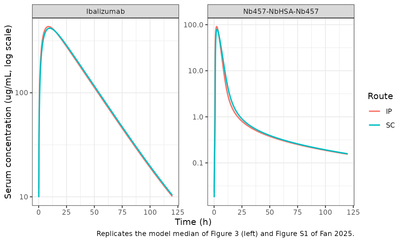
nbIp <- filter(mousePk, drug == "Nb457-NbHSA-Nb457", route == "IP")
nbSc <- filter(mousePk, drug == "Nb457-NbHSA-Nb457", route == "SC")
at   <- function(d, t) approx(d$time, d$Cc, t)$y

anchors <- data.frame(
  Quantity = c("IP peak", "SC peak", "IP 24 h", "IP 72 h", "IP 120 h"),
  `Figure 3 median` = c(81, 77, 0.9, 0.27, 0.16),
  Simulated = signif(c(
    max(nbIp$Cc), max(nbSc$Cc), at(nbIp, 24), at(nbIp, 72), at(nbIp, 120)
  ), 3),
  check.names = FALSE
)
anchors$`% diff` <- round(
  (anchors$Simulated - anchors$`Figure 3 median`) /
    anchors$`Figure 3 median` * 100, 1
)
knitr::kable(anchors, caption = "Model median against values digitized from Figure 3 (left).")| Quantity | Figure 3 median | Simulated | % diff |
|---|---|---|---|
| IP peak | 81.00 | 91.200 | 12.6 |
| SC peak | 77.00 | 79.300 | 3.0 |
| IP 24 h | 0.90 | 0.845 | -6.1 |
| IP 72 h | 0.27 | 0.262 | -3.0 |
| IP 120 h | 0.16 | 0.154 | -3.8 |
# Every anchor within 15 percent of the digitized published median.
stopifnot(all(abs(anchors$`% diff`) < 15))
The packaged model reproduces the published median of Figure 3 to
within the precision with which that figure can be read. Note that the
model median sits well below the observed peak
concentrations in that same panel: the highest observed dot is near
exp(5.6) = 270 ug/mL against a median of 81 ug/mL. That
under-prediction of the peak is a property of the published fit, not of
this transcription, and it explains most of the NCA discrepancy
below.
Murine PK: NCA against the published summary
The Results section reports observed-data NCA for both drugs and both routes. To compare like with like, the simulated profiles are sampled on exactly the published sampling grid (0, 1, 4, 8, 12, 24, 72, 120 h) before running PKNCA, so the simulated Cmax is subject to the same grid-resolution loss as the observed Cmax.
obsGrid <- c(0, 1, 4, 8, 12, 24, 72, 120)

ncaConc <- bind_rows(lapply(
  list(
    list(mod = zNb,  drug = "Nb457-NbHSA-Nb457", route = "IP", cmt = "depot_ip"),
    list(mod = zNb,  drug = "Nb457-NbHSA-Nb457", route = "SC", cmt = "depot_sc"),
    list(mod = zIba, drug = "Ibalizumab",        route = "IP", cmt = "depot_ip"),
    list(mod = zIba, drug = "Ibalizumab",        route = "SC", cmt = "depot_sc")
  ),
  function(a) {
    s <- solveIt(a$mod, evt(0, 400, a$cmt, obsGrid))
    data.frame(
      id = 1L, treatment = paste(a$drug, a$route),
      time = s$time, Cc = s$Cc
    )
  }
)) |>
  filter(!is.na(Cc))
#> ℹ omega/sigma items treated as zero: 'etalcl', 'etalvc'
#> ℹ omega/sigma items treated as zero: 'etalcl', 'etalvc'
#> ℹ omega/sigma items treated as zero: 'etalcl', 'etalvc'
#> ℹ omega/sigma items treated as zero: 'etalcl', 'etalvc'

ncaDose <- data.frame(
  id = 1L, treatment = unique(ncaConc$treatment), time = 0, dose = 400
)

ncaRes <- PKNCA::pk.nca(PKNCA::PKNCAdata(
  PKNCA::PKNCAconc(ncaConc, Cc ~ time | treatment + id),
  PKNCA::PKNCAdose(ncaDose, dose ~ time | treatment + id),
  intervals = data.frame(
    start = 0, end = 120,
    cmax = TRUE, tmax = TRUE, auclast = TRUE, half.life = TRUE
  )
))

published <- data.frame(
  treatment = c(
    "Nb457-NbHSA-Nb457 IP", "Nb457-NbHSA-Nb457 SC",
    "Ibalizumab IP", "Ibalizumab SC"
  ),
  cmax      = c(175.5, 67.04, 315.3, 251.5),
  half.life = c(7.47, 27.71, 24.75, 34.31)
)

ncaTbl <- nlmixr2lib::ncaComparisonTable(
  as.data.frame(ncaRes), published,
  by = "treatment",
  params = c("cmax", "half.life"),
  units = c(cmax = "ug/mL", half.life = "h")
)
knitr::kable(ncaTbl, caption = "Simulated NCA versus the observed-data NCA reported in the Results section.")| NCA parameter | treatment | Reference | Simulated | % diff |
|---|---|---|---|---|
| Cmax (ug/mL) | Nb457-NbHSA-Nb457 IP | 176 | 64.3 | -63.4%* |
| Cmax (ug/mL) | Nb457-NbHSA-Nb457 SC | 67 | 65.1 | -2.8% |
| Cmax (ug/mL) | Ibalizumab IP | 315 | 431 | +36.8%* |
| Cmax (ug/mL) | Ibalizumab SC | 252 | 411 | +63.4%* |
| t½ (h) | Nb457-NbHSA-Nb457 IP | 7.47 | 39.2 | +424.2%* |
| t½ (h) | Nb457-NbHSA-Nb457 SC | 27.7 | 36.8 | +32.8%* |
| t½ (h) | Ibalizumab IP | 24.8 | 19.9 | -19.4% |
| t½ (h) | Ibalizumab SC | 34.3 | 19.9 | -42.1%* |
attr(ncaTbl, "footnote")
#> [1] "* differs from reference by more than ±20%."
Only two of the eight cells fall inside 20%: the nanobody SC Cmax (65.1 versus 67.0 ug/mL, -2.8%) and the ibalizumab IP half-life (19.9 versus 24.8 h, -19.4%). The nanobody IP Cmax is under-predicted by a factor of 2.7 and both ibalizumab Cmax values are over-predicted by 37-63%.
The half-life rows deserve a separate note, because the gap there is
structural rather than numerical. A one-compartment model whose
absorption is faster than its elimination has a single terminal slope,
so its half-life cannot depend on the route: the simulated values are
39.2 h (IP) and 36.8 h (SC) for the nanobody, and 19.9 h by both routes
for ibalizumab. The published observed-data NCA instead reports 7.47 h
versus 27.71 h for the nanobody and 24.75 h versus 34.31 h for
ibalizumab – a 3.7-fold and a 1.4-fold route difference for the same
drug. No model of the published structure can produce a route-dependent
terminal half-life, so those reference values reflect the sparse design
(n = 4, eight time points, a 120 h window) rather than a
target the packaged model could have been expected to hit.
The reference column throughout is an NCA of the observed mouse data, while the simulated column is the model’s own typical-value prediction; the published visual predictive check in Figure 3 shows the same gap, with the model median running below the observed peaks. These rows therefore measure a limitation of the published fit rather than a transcription error, and no parameter was adjusted to close them.
Murine PD: viral load under the four-dose regimen
The PD arm received 400 ug IP on day 1 followed by 400 ug SC on days 3, 5 and 7, with viral load followed to week 4. Figure 3 (right) and Figure 2 (right) show a control arm rising steeply and a treated arm rising far more slowly.
pdDoses <- function() {
  obsTimes <- seq(0, 28 * 24, by = 6)
  ipEv  <- evt(24, 400, "depot_ip", obsTimes)
  scEv  <- data.frame(
    id = 1L, time = c(3, 5, 7) * 24, amt = 400, evid = 1L,
    cmt = "depot_sc", dvid = NA_integer_
  )
  ev <- rbind(ipEv, scEv)
  ev[order(ev$time, -ev$evid), ]
}

mousePd <- bind_rows(lapply(
  list(
    list(mod = zNb,  drug = "Nb457-NbHSA-Nb457"),
    list(mod = zIba, drug = "Ibalizumab")
  ),
  function(a) {
    obsTimes <- seq(0, 28 * 24, by = 6)
    tx  <- solveIt(a$mod, pdDoses())
    ctl <- solveIt(a$mod, evt(numeric(0), 0, "depot_sc", obsTimes))
    bind_rows(
      data.frame(drug = a$drug, arm = "Treated", time = tx$time,  virus = tx$virus),
      data.frame(drug = a$drug, arm = "Control", time = ctl$time, virus = ctl$virus)
    )
  }
))
#> ℹ omega/sigma items treated as zero: 'etalcl', 'etalvc'
#> ℹ omega/sigma items treated as zero: 'etalcl', 'etalvc'
#> ℹ omega/sigma items treated as zero: 'etalcl', 'etalvc'
#> ℹ omega/sigma items treated as zero: 'etalcl', 'etalvc'

ggplot(filter(mousePd, virus > 0), aes(time / 168, virus, colour = arm)) +
  geom_line(linewidth = 0.8) +
  facet_wrap(~drug) +
  scale_y_continuous(trans = "log10") +
  labs(
    x = "Time (weeks post-infection)", y = "Viral load (copies/mL, log scale)",
    colour = "Arm",
    caption = "Structure of Figure 3 (right); absolute magnitudes do not reproduce - see Errata."
  ) +
  theme_bw()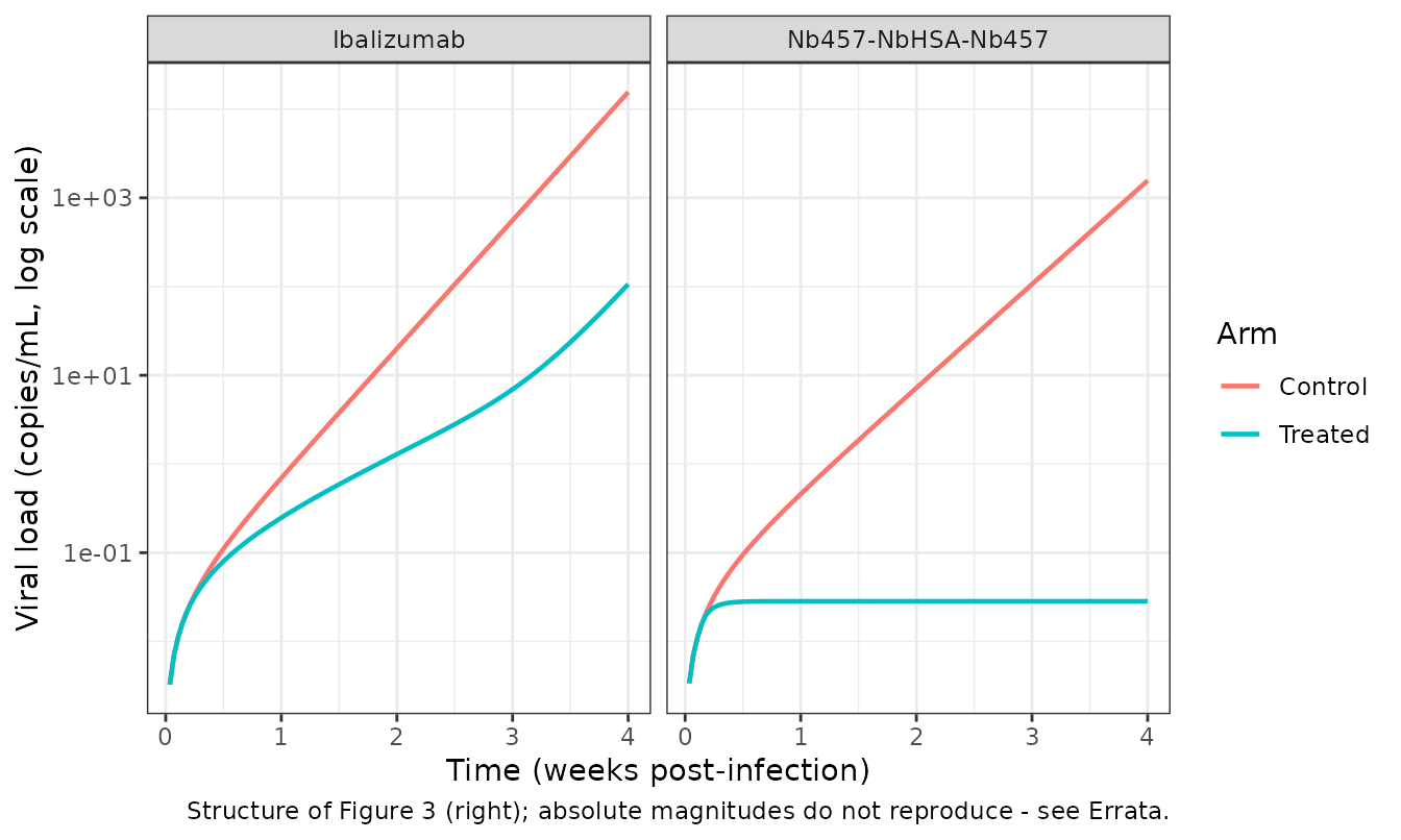
pdWeeks <- mousePd |>
  filter(time %in% (c(1, 2, 3, 4) * 168)) |>
  mutate(week = time / 168) |>
  select(drug, arm, week, virus) |>
  pivot_wider(names_from = week, values_from = virus, names_prefix = "week ") |>
  mutate(across(starts_with("week"), ~ signif(.x, 3)))
knitr::kable(pdWeeks, caption = "Simulated viral load (copies/mL) at the four published sampling weeks.")| drug | arm | week 1 | week 2 | week 3 | week 4 |
|---|---|---|---|---|---|
| Nb457-NbHSA-Nb457 | Treated | 0.0283 | 0.0283 | 0.0283 | 2.83e-02 |
| Nb457-NbHSA-Nb457 | Control | 0.4590 | 7.2000 | 106.0000 | 1.56e+03 |
| Ibalizumab | Treated | 0.2480 | 1.2900 | 6.9400 | 1.06e+02 |
| Ibalizumab | Control | 0.6940 | 20.0000 | 558.0000 | 1.55e+04 |
The shape is reproduced: the untreated arm grows
log-linearly, the nanobody arm is driven down (its fitted
Imax = 1.963 exceeds 1, so a free concentration above
IC50 / (Imax - 1) = 0.0354 ug/mL makes the expansion term
negative), and the ibalizumab arm, whose Imax = 0.42, only
slows growth. The magnitudes do not reproduce: Figure 3
(right) puts the control median at about exp(5.8) = 3e2
copies/mL at week 1 and exp(15.6) = 6e6 at week 4, against
a simulated 0.5 and 1.6e3. This gap is examined in the Errata; it is
present identically in the human simulations below and for both drugs,
so it is a property of the published parameter set rather than of a
single table row.
nbPd <- filter(mousePd, drug == "Nb457-NbHSA-Nb457", time == 4 * 168)
ibPd <- filter(mousePd, drug == "Ibalizumab",        time == 4 * 168)

# Both drugs suppress relative to their own control at week 4, and the
# nanobody (Imax > 1) suppresses by orders of magnitude more than
# ibalizumab (Imax < 1) - the paper's central mechanistic claim.
nbRatio <- nbPd$virus[nbPd$arm == "Treated"] / nbPd$virus[nbPd$arm == "Control"]
ibRatio <- ibPd$virus[ibPd$arm == "Treated"] / ibPd$virus[ibPd$arm == "Control"]
c(nanobody_treated_over_control = signif(nbRatio, 3),
  ibalizumab_treated_over_control = signif(ibRatio, 3))
#>   nanobody_treated_over_control ibalizumab_treated_over_control
#>                        1.81e-05                        6.84e-03

stopifnot(nbRatio < 1e-3, ibRatio < 1, nbRatio < ibRatio)
Human PK: replicating Figure 4
Figure 4 simulates 20 mg/kg SC once every 2 days for four doses in a human. The published trace peaks near 155 ug/mL after the first dose and near 218 ug/mL after each of the following three, showing the “slight accumulation” the Results describe, and returns to baseline by about day 8.
doseMg  <- 20 * 70
humanPk <- solveIt(
  zHNb,
  evt(c(0, 2, 4, 6) * 24, doseMg, "depot_sc", seq(0, 11 * 24, by = 0.1)),
  params = c(WT = 70)
)
#> ℹ omega/sigma items treated as zero: 'etalcl', 'etalvc'

ggplot(humanPk, aes(time / 24, Cc)) +
  geom_line(colour = "blue", linewidth = 0.7) +
  labs(
    x = "Time (Days)", y = "Nb457-NbHSA-Nb457 Conc (ug/mL)",
    caption = "Replicates Figure 4 of Fan 2025 (20 mg/kg SC once every 2 days, four doses)."
  ) +
  theme_bw()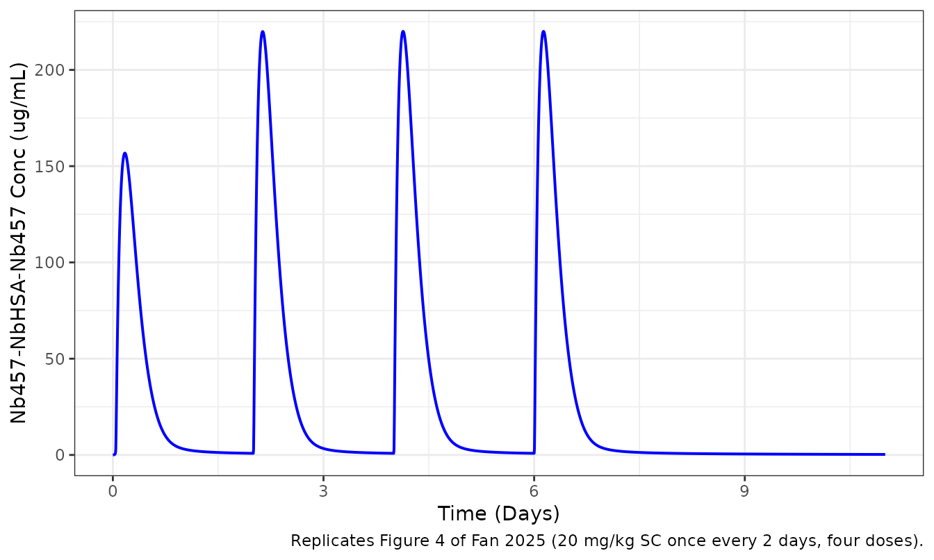
peakIn <- function(a, b) max(humanPk$Cc[humanPk$time >= a & humanPk$time < b])
fig4 <- data.frame(
  Dose = 1:4,
  `Figure 4 peak` = c(155, 218, 218, 218),
  Simulated = signif(vapply(0:3, function(k) peakIn(k * 48, k * 48 + 48), 0), 4),
  check.names = FALSE
)
fig4$`% diff` <- round(
  (fig4$Simulated - fig4$`Figure 4 peak`) / fig4$`Figure 4 peak` * 100, 1
)
knitr::kable(fig4, caption = "Peak concentration per dose interval against Figure 4.")| Dose | Figure 4 peak | Simulated | % diff |
|---|---|---|---|
| 1 | 155 | 156.8 | 1.2 |
| 2 | 218 | 219.9 | 0.9 |
| 3 | 218 | 220.0 | 0.9 |
| 4 | 218 | 220.0 | 0.9 |
# All four peaks within 5 percent of the digitized published trace.
stopifnot(all(abs(fig4$`% diff`) < 5))
This is the strongest validation available for the packaged system:
it exercises the QE-TMDD algebra, both absorption depots, the allometric
scaling of CL and V3, and the 70 kg reference
anchor simultaneously, and every peak lands within 5% of the published
trace.
Human PD: replicating Figure 5
Figure 5 compares three regimens - 20 mg/kg every 2 days, 20 mg/kg
once daily and 40 mg/kg every 2 days, each for one month - against an
untreated control. Its notable feature is that the three treated traces
are visually indistinguishable, because free concentrations stay far
above the fixed IC50 = 0.0341 ug/mL throughout in every
regimen.
regimens <- list(
  list(label = "Control",       times = numeric(0),                     amt = 0),
  list(label = "20 mg/kg q2d",  times = seq(0, by = 48, length.out = 14), amt = 20 * 70),
  list(label = "20 mg/kg qd",   times = seq(0, by = 24, length.out = 28), amt = 20 * 70),
  list(label = "40 mg/kg q2d",  times = seq(0, by = 48, length.out = 14), amt = 40 * 70)
)
obsTimes <- seq(0, 28 * 24, by = 6)

humanPd <- bind_rows(lapply(regimens, function(r) {
  s <- solveIt(
    zHNb, evt(r$times, r$amt, "depot_sc", obsTimes), params = c(WT = 70)
  )
  data.frame(regimen = r$label, time = s$time, virus = s$virus)
}))
#> ℹ omega/sigma items treated as zero: 'etalcl', 'etalvc'
#> ℹ omega/sigma items treated as zero: 'etalcl', 'etalvc'
#> ℹ omega/sigma items treated as zero: 'etalcl', 'etalvc'
#> ℹ omega/sigma items treated as zero: 'etalcl', 'etalvc'

ggplot(filter(humanPd, virus > 0), aes(time / 168, virus, colour = regimen)) +
  geom_line(linewidth = 0.8) +
  scale_y_continuous(trans = "log10") +
  labs(
    x = "Time (Weeks)", y = "Viral load (copies/mL, log scale)", colour = "Regimen",
    caption = "Structure of Figure 5 of Fan 2025; absolute magnitudes do not reproduce - see Errata."
  ) +
  theme_bw()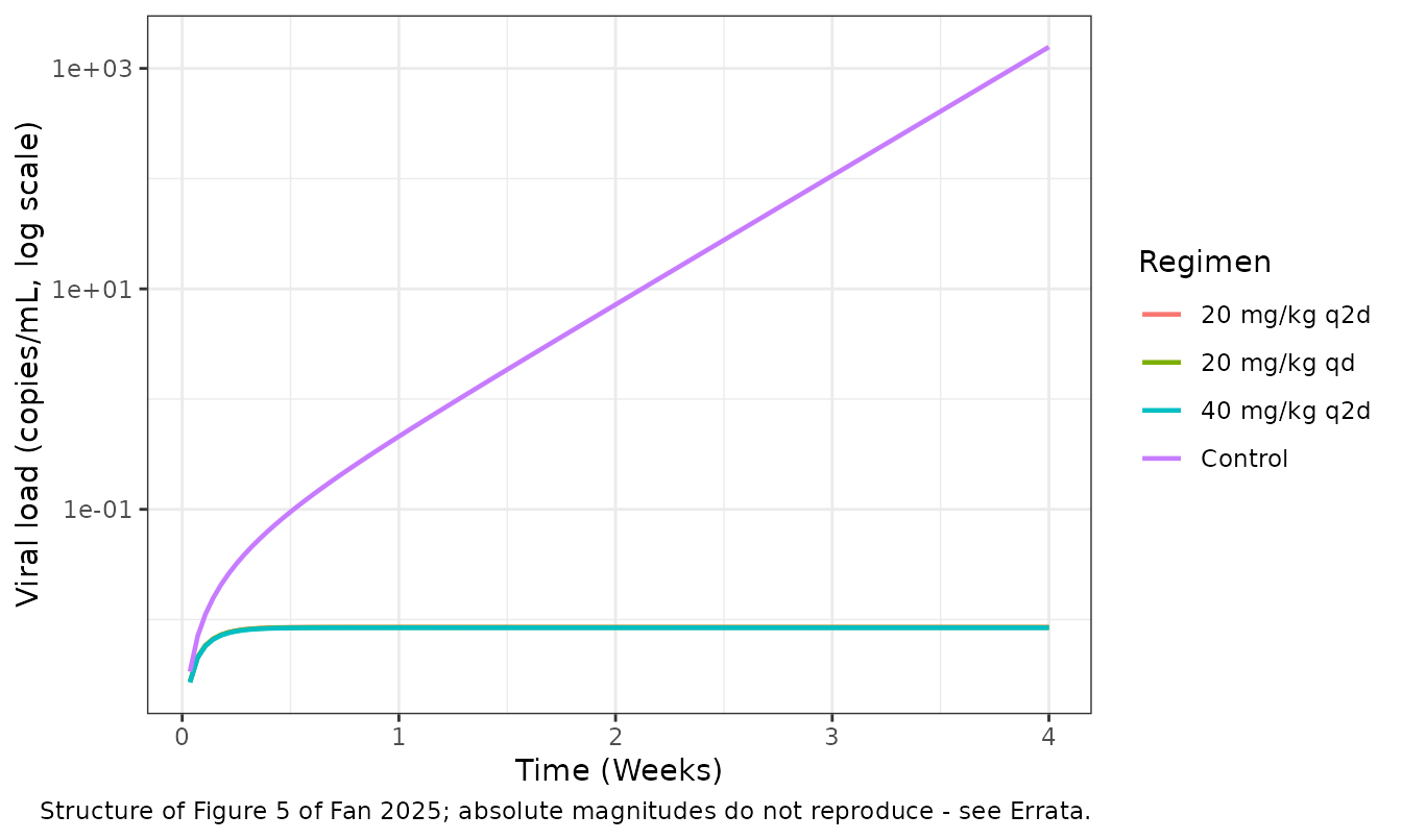
wk4 <- humanPd |>
  filter(time == 4 * 168) |>
  select(regimen, virus)
knitr::kable(
  mutate(wk4, virus = signif(virus, 3)),
  caption = "Simulated viral load at week 4 by regimen."
)| regimen | virus |
|---|---|
| Control | 1.56e+03 |
| 20 mg/kg q2d | 8.53e-03 |
| 20 mg/kg qd | 8.49e-03 |
| 40 mg/kg q2d | 8.42e-03 |
treated <- wk4$virus[wk4$regimen != "Control"]
control <- wk4$virus[wk4$regimen == "Control"]

# The paper's Figure 5 claim: the three treated traces are superimposed, and
# all are far below control.
stopifnot(
  max(treated) / min(treated) < 1.05,
  max(treated) < control / 1000
)
signif(c(spread = max(treated) / min(treated), suppression = control / max(treated)), 3)
#>      spread suppression
#>    1.01e+00    1.83e+05
The qualitative conclusion of Figure 5 is reproduced exactly: the three regimens are within 1% of each other at week 4 and all sit orders of magnitude below the untreated control. The claim in the Discussion that “increasing dose intensity had a more pronounced effect on HIV-1 inhibition than increasing the total dose amount” is not discernible in either the published figure or this replication - all three curves overlie because the drug effect is saturated.
Human PK: the ibalizumab validation leg
Figure S7 overlays the projected ibalizumab profile on observed clinical concentrations. Table S2 gives the regimen as “weekly 10 mg/kg IV infusions for the first 9 doses, followed by 10 mg/kg infusions q2wk”, with trough PK samples at every visit through week 48. This is the only leg of the extrapolation with real human data behind it.
Table S2 does not state an infusion duration, so each dose is given
here as an intravenous bolus into central. The simulated
peak is therefore an upper bound on what any finite infusion would
produce, and the peak row of the table below should be read with that in
mind; the trough rows are unaffected.
ibaTimes <- c(
  seq(0, by = 168, length.out = 9),
  seq(8 * 168 + 336, by = 336, length.out = 20)
)
ibaTimes <- ibaTimes[ibaTimes <= 48 * 168]
# Pre-dose trough samples sit 0.01 h before each dose after the first; the
# t = 0 dose has no pre-dose sample to take (subtracting there would ask for a
# negative time).
ibaObs   <- sort(unique(c(
  seq(0, 48 * 168, by = 6), ibaTimes[ibaTimes > 0] - 0.01
)))
ibaSim   <- solveIt(
  zHIba,
  evt(ibaTimes, 10 * 70, "central", ibaObs),
  params = c(WT = 70)
) |>
  filter(!is.na(Cc))
#> ℹ omega/sigma items treated as zero: 'etalcl', 'etalvc'

ggplot(ibaSim, aes(time / 168, Cc)) +
  geom_line(colour = "salmon", linewidth = 0.5) +
  labs(
    x = "Time (Weeks)", y = "Ibalizumab Conc (ug/mL)",
    caption = "Compare Figure S7 of Fan 2025 (10 mg/kg arm)."
  ) +
  theme_bw()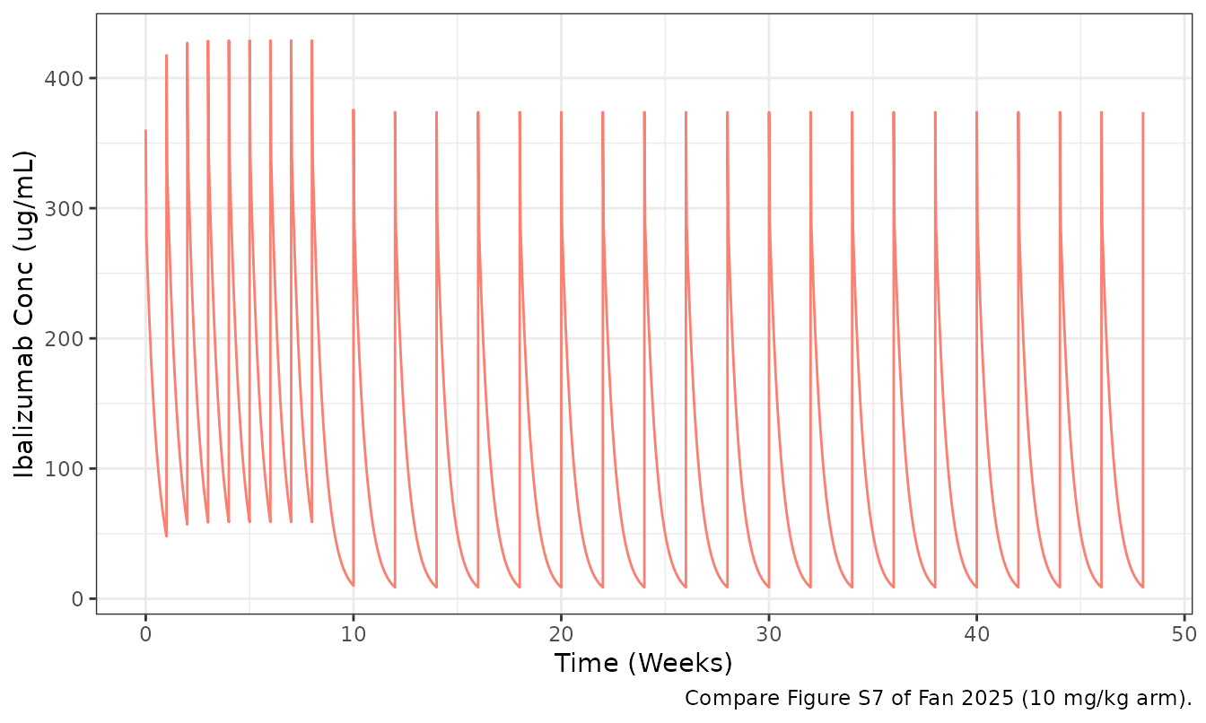
troughAt <- function(t) ibaSim$Cc[which.min(abs(ibaSim$time - (t - 0.01)))]
ibaTbl <- data.frame(
  Quantity = c(
    "Peak after dose 1", "Trough, weekly phase (week 8)",
    "Trough, q2w phase (week 24)", "Trough, q2w phase (week 48)"
  ),
  `Figure S7 model line` = c(225, 30, 28, 28),
  `Figure S7 observed`   = c(NA, 163, 37, 47),
  Simulated = signif(c(
    max(ibaSim$Cc[ibaSim$time < 168]), troughAt(8 * 168),
    troughAt(24 * 168), troughAt(48 * 168)
  ), 3),
  check.names = FALSE
)
knitr::kable(ibaTbl, caption = "Packaged ibalizumab projection against values digitized from Figure S7.")| Quantity | Figure S7 model line | Figure S7 observed | Simulated |
|---|---|---|---|
| Peak after dose 1 | 225 | NA | 360.00 |
| Trough, weekly phase (week 8) | 30 | 163 | 58.90 |
| Trough, q2w phase (week 24) | 28 | 37 | 8.68 |
| Trough, q2w phase (week 48) | 28 | 47 | 8.68 |
The packaged projection has too much peak-to-trough swing: it peaks
60% above the published line (360 versus 225 ug/mL), sits about twice as
high at the week-8 trough while doses are still weekly (58.9 versus 30
ug/mL), and then falls about three-fold below it once dosing widens to
every two weeks (8.68 versus 28 ug/mL at weeks 24 and 48). A profile
that is simultaneously high at the short inter-dose interval and low at
the long one is the signature of a terminal slope that is too steep. The
implied terminal half-life of the published curve (falling from roughly
155 to 28 ug/mL over a 14-day interval) is about 5.7 days, against 2.7
days for ln(2) * Vss / CL with the parameters here. Part of
the peak excess is the bolus assumption noted above, but that cannot
explain the trough behaviour. Q and V4 are the
only human parameters the paper does not print, so they are the natural
suspects; see Errata. They were derived by applying the published
exponents to the published murine values and were not
adjusted to close this gap.
Assumptions and deviations
-
Reference body weight (70 kg) and murine body weight (0.02
kg) are not printed anywhere in the paper. Both are recoverable
from its own arithmetic: the reported human
V3of 36.26 mL/kg divided into the murine 0.73 mL gives 0.0201 kg, and 26.9 mL/kg into 0.54 mL gives 0.0201 kg; scaling the murineCLof 0.69 mL/h by(70 / 0.02)^0.85and dividing by 70 kg reproduces the published 10.21 mL/h/kg to 0.6%, and the same operation on ibalizumab reproduces 0.35 mL/h/kg exactly. The human files anchor at 70 kg with the published exponents as fixede_wt_*terms. -
Ibalizumab human
QandV4are not printed. They are derived by applying the published exponents (0.85 on clearances, 1 on volumes) to the murine Table 1 values, giving 1.915 L/h and 0.420 L. The paper says only that “we only scaled CL and V”. -
Two-compartment ibalizumab peripheral exchange is
declared by the Table 1 footnote but the modified eq 3 is never printed.
This implementation drives distribution with the free
central concentration
Cc, the species available to leave the vascular space, consistent with the QE-TMDD formulation of eqs 3-5. -
ksynis derived, not tabulated: eq 4 withA4(0) = RTOT0at steady state forcesksyn = kdeg * RTOT0. -
IIV in the human projections is carried over from
the murine fit. The paper’s human figures are deterministic; use
rxode2::zeroRe()(as this vignette does throughout) to reproduce them. -
Residual error and IIV are on the variance scale.
Table 1 footnote a states that “RSE for omega and sigma are reported on
the approximate S.D. scale (standard error/variance estimate)/2”, which
identifies the tabulated estimates as NONMEM variances. The nlmixr2
propSd/addSdparameters are SDs, so they are entered as square roots. - The IP depot is retained in the human files even though only SC (and, for ibalizumab, IV) dosing was simulated, so that the packaged structure matches the murine model it was scaled from.
-
Ibalizumab clinical doses are simulated as IV
boluses. Table S2 specifies “IV infusions” but gives no
infusion duration, and none is recoverable from the paper, so no
dur/rateis set. This inflates the simulated peak relative to Figure S7 and leaves the troughs unchanged.
Errata and unresolved discrepancies
-
The PD layer does not reproduce the published viral-load magnitudes. Using the Table 2 parameters verbatim in eqs 6-7, the untreated control reaches roughly 0.5, 7, 1e2 and 1.6e3 copies/mL at weeks 1-4. Figure 3 (right) plots the murine control on a natural-log axis at about 5.8, 9.5, 12.6 and 15.6, i.e. 3e2, 1.3e4, 3e5 and 6e6 copies/mL, and Figure 5 (left) puts the human control at about 1e2, 1e4, 3e5 and 1e7. The published control is therefore several hundred-fold above the packaged prediction at week 1, growing to several thousand-fold by week 4.
The gap decomposes cleanly into a scale error and a slope error, and the scale part has a very likely explanation. Table 2 gives
BASE Tas 814.2 cells/mL. A CD4+ T-cell count of 814 cells/mL is 0.8 cells/uL, which is not a viable value; 814 cells/uL is an unremarkable normal CD4 count. The units cell is almost certainly mislabelled by a factor of- Because eqs 6-7 are linear in
A5,virusis exactly proportional toBASE_T, so this is testable without touching the fit:
- Because eqs 6-7 are linear in
wkT   <- c(1, 2, 3, 4) * 168
ctlEv <- evt(numeric(0), 0, "depot_sc", seq(0, 28 * 24, by = 6))
asIs  <- solveIt(zNb, ctlEv)
#> ℹ omega/sigma items treated as zero: 'etalcl', 'etalvc'
perUl <- solveIt(zNb, ctlEv, params = c(lrbase_infected = log(814.2 * 1000)))
#> ℹ omega/sigma items treated as zero: 'etalcl', 'etalvc'

at2 <- function(s) approx(s$time, s$virus, wkT)$y
# Figure 3 (right), murine control, read off the natural-log axis.
pubFig3 <- exp(c(5.8, 9.5, 12.6, 15.6))

baseT <- data.frame(
  Week = 1:4,
  `As published (cells/mL)` = signif(at2(asIs), 3),
  `Reading BASE_T as cells/uL` = signif(at2(perUl), 3),
  `Figure 3 control` = signif(pubFig3, 3),
  check.names = FALSE
)
baseT$`Fold gap, as published`  <- signif(pubFig3 / at2(asIs), 3)
baseT$`Fold gap, as cells/uL`   <- signif(pubFig3 / at2(perUl), 3)
knitr::kable(baseT, caption = "Effect of reading BASE_T as cells/uL rather than cells/mL.")| Week | As published (cells/mL) | Reading BASE_T as cells/uL | Figure 3 control | Fold gap, as published | Fold gap, as cells/uL |
|---|---|---|---|---|---|
| 1 | 0.459 | 459 | 330 | 720 | 0.72 |
| 2 | 7.200 | 7200 | 13400 | 1860 | 1.86 |
| 3 | 106.000 | 106000 | 297000 | 2790 | 2.79 |
| 4 | 1560.000 | 1560000 | 5960000 | 3810 | 3.81 |
# virus is exactly linear in BASE_T, so the rescale is a pure factor of 1000.
stopifnot(isTRUE(all.equal(at2(perUl) / at2(asIs), rep(1000, 4))))
As published the model sits 720- to 3,800-fold below the digitized
control; reading BASE_T as cells/uL brings it to within a
factor of 1.4 at week 1 and 3.8 at week 4. What remains after that
rescale is a pure slope difference, and no prefactor can absorb it: in
eqs 6-7 the asymptotic log-slope of virus is exactly
kPV - kCV, which for the nanobody is 0.016 /h = 2.69
natural-log units per week, against about 3.3 read off Figure 3 (right)
and about 3.8 off Figure 5 (left). Notably, the ibalizumab row
of Table 2 gives kPV - kCV = 0.0198 /h = 3.33 log units per
week, which matches the Figure 3 control slope well – yet the two drugs
share the same experimental control arm, so the two fits disagree about
a curve they both observed.
The packaged files keep 814.2 exactly as Table 2 prints
it. The rescale above is a diagnostic, not a correction: the
units error is inferred rather than stated, and beta,
lambda and BASE_T enter the viral-load
prediction only through their product, so a reader who wants the
published figure magnitudes can supply any one of the three. No value
was altered.
The shape of every PD figure is reproduced faithfully:
log-linear untreated growth after an initial transient from
virus(0) = 0, a treated arm held far below control, and
three superimposed human regimens. 2. The ibalizumab human
projection decays too fast relative to Figure S7 (2.7-day
versus about 5.7-day terminal half-life). The symptom is excess
peak-to-trough swing rather than a uniform offset: the peak is about 60%
high, the week-8 trough about twice high while dosing is weekly, and the
week-24 and week-48 troughs about three-fold low once dosing widens to
every two weeks. The unprinted Q and V4 are
the only degrees of freedom, and no published value constrains them, so
the principled derivation was kept rather than back-solved from the
figure. 3. The abstract’s precision claim is contradicted by
Table 1. The abstract and Results both state that “all model
parameters were estimated with high precision, with relative standard
errors below 50%”, but the ibalizumab target parameters carry %RSE of
249.6 (RTOT0), 308.5 (K M) and 1121
(k INT). The ibalizumab target-mediated limb should be
treated as essentially unidentified. 4. Table 1 mislabels the
ibalizumab residual-error row. The row sits in the Ibalizumab
block but its Description cell reads “Proportional error of Nb 457 -Nb
HSA -Nb 457”. It is read here as the ibalizumab proportional error. 5.
The naive-pooled statement conflicts with the reported
IIV. The Methods state that “the interindividual variabilities
(IIVs) for the fixed-effect parameters were not preserved”, yet Table 1
reports omega CL and omega V3 with RSEs for
both drugs. The tabulated variances are carried in the model files,
since they are concrete estimates with reported precision;
zeroRe() recovers the pooled typical-value behaviour. 6.
lambda is defined in the direction opposite to its
use. The text defines lambda as “the ratio of infected T cells
to HIV viral load”, but eq 7 drives virus toward
lambda * infected, which makes it the ratio of viral load
to infected cells. The equation is implemented as printed. 7.
IC50 versus SC50. Equation 6
and Figure 1 use SC50; Table 2 labels the nanobody row
IC 50 and the ibalizumab row SC 50. They are
the same quantity; both model files use the canonical name
lic50. 8. Two sampling-schedule descriptions
differ. The Materials and Methods describe the PK study as a
single 400 ug IP or SC dose on day 1, while Table S1 lists the
full four-dose regimen against both the PK and PD sampling columns. The
single-dose reading is used for the PK simulations here, consistent with
the 0-120 h post-dose sampling window and with the separate-animals
design. 9. A correction notice exists but does not touch the
model. The article was published on 19 September 2025 and
corrected on 4 November 2025 for an error in the Acknowledgments; no
parameter, equation or figure is affected.